Models

2024-10-24

The main functions of the StormR package, spatialBehaviour() and temporalBehaviour(), allow to compute characteristics of the storm surface wind field, as re-constructed from storm track data and a parametric cyclone model. Three parametric models are implemented in this package: Holland (1980), Willoughby et al. (2006), and Boose et al. (2004). The use of one model or the other is defined using the method argument in spatialBehaviour() and temporalBehaviour() functions.

The original Holland (1980) and Willoughby et al. (2006) models provide a symmetrical wind field around the cyclone centre. However, cyclonic winds are not symmetric, and an order zero asymmetry is caused by the storm translation (forward motion). We therefore suggest using an asymmetric version of the parametric wind fields that takes into account storm motion. In the StormR package the methods developed by Miyazaki et al. (1962) and Chen (1994) that allow to take this asymmetry into account can be used to adjust the outputs of the symmetrical models accordingly. These can be activated by using the asymmetry argument of the spatialBehaviour() and temporalBehaviour() functions. The model of Boose et al. (2004) is already an asymmetrical version of the Holland (1980) model. Contrary to the Holland (1980) and Willoughby et al. (2006), this model considers different parameter settings over water or over lands.

By default the spatialBehaviour() and temporalBehaviour() functions use the Willoughby et al. (2006) model adjusted using the Chen (1994) method.

Holland (1980) symmetric wind field

The Holland model (1980), widely used in the literature, is based on the gradient wind balance in mature tropical cyclones. The wind speed distribution is computed from the circular air pressure field, which can be derived from the central and environmental pressure and the radius of maximum winds.

$$v_r = \sqrt{\frac{b}{\rho} \times \left(\frac{R_m}{r}\right)^b \times (p_{oci} - p_c) \times e^{-\left(\frac{R_m}{r}\right)^b} + \left(\frac{r \times f}{2}\right)^2} - \left(\frac{r \times f}{2}\right)$$

with, $$b = \frac{\rho \times e \times v_m^2}{p_{oci} - p_c}$$$$f = 2 \times 7.29 \times 10^{-5} \sin(\phi)$$

where,
$v_r$ is the tangential wind speed (in $m.s^{-1}$),
$b$ is the shape parameter,
$\rho$ is the air density set to $1.15 kg.m^{-3}$,
$e$ is the base of natural logarithms (~2.718282),
$v_m$ the maximum sustained wind speed (in $m.s^{-1}$),
$p_{oci}$ is the pressure at outermost closed isobar of the storm (in $Pa$),
$p_c$ is the pressure at the centre of the storm (in $Pa$),
$r$ is the distance to the eye of the storm (in $km$),
$R_m$ is the radius of maximum sustained wind speed (in $km$),
$f$ is the Coriolis force (in $N.kg^{-1}$), and
$\phi$ is the latitude.

Willoughby et al. (2006) symmetric wind field

The Willoughby et al. (2006) model is an empirical model fitted to aircraft observations. The model considers two regions: inside the eye and at external radii, for which the wind formulations use different exponents to better match observations. In this model, the wind speed increases as a power function of the radius inside the eye and decays exponentially outside the eye after a smooth polynomial transition across the eyewall (see also Willoughby (1995), Willoughby et al. (2004)).

$$\left\{ \begin{aligned} v_r &= v_m \times \left(\frac{r}{R_m}\right)^{n} \quad if \quad r < R_m \\ v_r &= v_m \times \left((1-A) \times e^{-\frac{|r-R_m|}{X1}} + A \times e^{-\frac{|r-R_m|}{X2}}\right) \quad if \quad r \geq R_m \\ \end{aligned} \right.$$

with, $$n = 2.1340 + 0.0077 \times v_m - 0.4522 \times \ln(R_m) - 0.0038 \times |\phi|$$$$X1 = 287.6 - 1.942 \times v_m + 7.799 \times \ln(R_m) + 1.819 \times |\phi|$$$$A = 0.5913 + 0.0029 \times v_m - 0.1361 \times \ln(R_m) - 0.0042 \times |\phi| \quad and \quad A\ge0$$

where,
$v_r$ is the tangential wind speed (in $m.s^{-1}$),
$v_m$ is the maximum sustained wind speed (in $m.s^{-1}$),
$r$ is the distance to the eye of the storm (in $km$),
$R_m$ is the radius of maximum sustained wind speed (in $km$),
$\phi$ is the latitude of the centre of the storm, and
$X2 = 25$.

Adding asymmetry to Holland (1980) and Willoughby et al. (2006) wind fields

The asymmetry caused by the translation of the storm can be added as follows,

$\vec{V} = \vec{V_c} + C \times \vec{V_t}$

where,
$\vec{V}$ is the combined, asymmetric wind field,
$\vec{V_c}$ is symmetric wind field,
$\vec{V_t}$ is the translation speed of the storm, and
$C$ is function of $r$, the distance to the eye of the storm (in $km$).

Two formulations of C proposed by Miyazaki et al. (1962) and Chen (1994) are implemented.

Miyazaki et al. (1962)

$C = e^{(-\frac{r}{500} \times \pi)}$

Chen (1994)

$C = \frac{3 \times R_m^{\frac{3}{2}} \times r^{\frac{3}{2}}}{R_m^3 + r^3 +R_m^{\frac{3}{2}} \times r^{\frac{3}{2}}}$

where,
$R_m$ is the radius of maximum sustained wind speed (in $km$).

Boose et al. (2004) asymmetric model

The Boose et al. (2004) model, or “HURRECON” model, is a modification of the Holland (1980) model (see also Boose et al. (2001)). In addition to adding asymmetry, this model treats of water and land differently, using different surface friction coefficient for each.

Wind speed

Wind speed is computed as follows,

$$v_r = F\left(v_m - S \times (1 - \sin(T)) \times \frac{v_h}{2} \right) \times \sqrt{\left(\frac{R_m}{r}\right)^b \times e^{1 - \left(\frac{R_m}{r}\right)^b}}$$

with, $$b = \frac{\rho \times e \times v_m^2}{p_{oci} - p_c}$$

where,
$v_r$ is the tangential wind speed (in $m.s^{-1}$),
$F$ is a scaling parameter for friction ($1.0$ in water, $0.8$ in land),
$v_m$ is the maximum sustained wind speed (in $m.s^{-1}$),
$S$ is a scaling parameter for asymmetry (usually set to $1$),
$T$ is the oriented angle (clockwise/counter clockwise in Northern/Southern Hemisphere) between the forward trajectory of the storm and a radial line from the eye of the storm to point $r$,
$v_h$ is the storm velocity (in $m.s^{-1}$),
$R_m$ is the radius of maximum sustained wind speed (in $km$),
$r$ is the distance to the eye of the storm (in $km$),
$b$ is the shape parameter,
$\rho = 1.15$ is the air density (in $kg.m^{-3}$),
$p_{oci}$ is the pressure at outermost closed isobar of the storm (in $Pa$), and
$p_c$ is the pressure at the centre of the storm ($pressure$ in $Pa$).

Wind direction

Wind direction is computed as follows,

$$\left\{ \begin{aligned} D = A_z - 90 - I \quad if \quad \phi > 0 \quad(Northern \quad Hemisphere) \\ D = A_z + 90 + I \quad if \quad \phi \leq 0 \quad(Southern \quad Hemisphere) \\ \end{aligned} \right.$$ where,
$D$ is the direction of the radial wind,
$A_z$ is the azimuth from point r to the eye of the storm,
$I$ is the cross isobar inflow angle ($20$ in water, $40$ in land), and
$\phi$ is the latitude.

Wind fields comparison

Here, we compare wind fields generated by different models that can be used in StormR for the same time and location (tropical cyclone Pam near Vanuatu)

sds <- defStormsDataset()

## Warning in checkInputsdefStormsDataset(filename, sep, fields, basin, seasons, : No basin argument specified. StormR will work as expected
##              but cannot use basin filtering for speed-up when collecting data

## === Loading data  ===
## Open database... /home/runner/work/_temp/Library/StormR/extdata/test_dataset.nc opened
## Collecting data ...
## === DONE ===

st <- defStormsList(sds = sds, loi = c(168.33, -17.73), names = "PAM", verbose = 0)
PAM <- getObs(st, name = "PAM")

pf <- spatialBehaviour(st, product = "Profiles", method = "Holland", asymmetry = "None", verbose = 0)
terra::plot(pf$PAM_Speed_41, main = "Holland (1980)", cex.main = 0.8, range = c(0, 90))
terra::plot(countriesHigh, add = TRUE)
lines(PAM$lon, PAM$lat, lty = 3)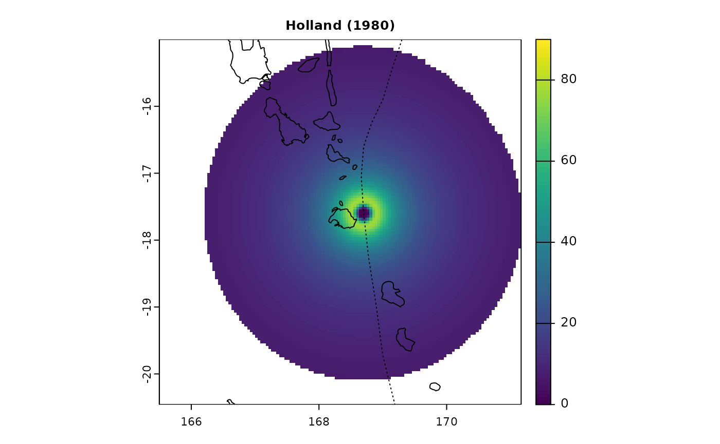

pf <- spatialBehaviour(st, product = "Profiles", method = "Willoughby", asymmetry = "None", verbose = 0)
terra::plot(pf$PAM_Speed_41, main = "Willoughby et al. (2006)", cex.main = 0.8, range = c(0, 90))
terra::plot(countriesHigh, add = TRUE)
lines(PAM$lon, PAM$lat, lty = 3)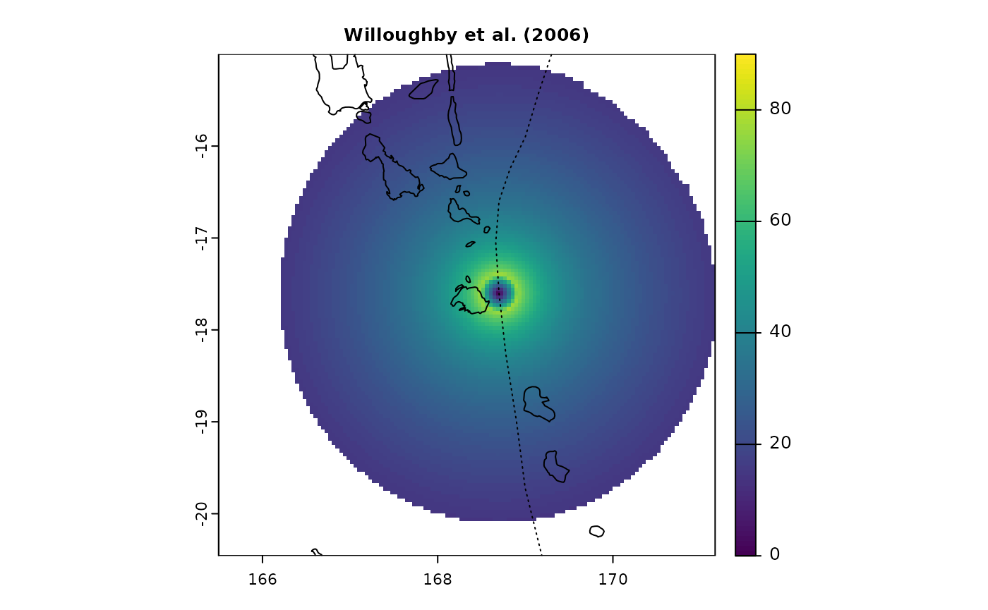

pf <- spatialBehaviour(st, product = "Profiles", method = "Holland", asymmetry = "Miyazaki", verbose = 0)
terra::plot(pf$PAM_Speed_41, main = "Holland (1980) + Miyazaki et al. (1962)", cex.main = 0.8, range = c(0, 90))
terra::plot(countriesHigh, add = TRUE)
lines(PAM$lon, PAM$lat, lty = 3)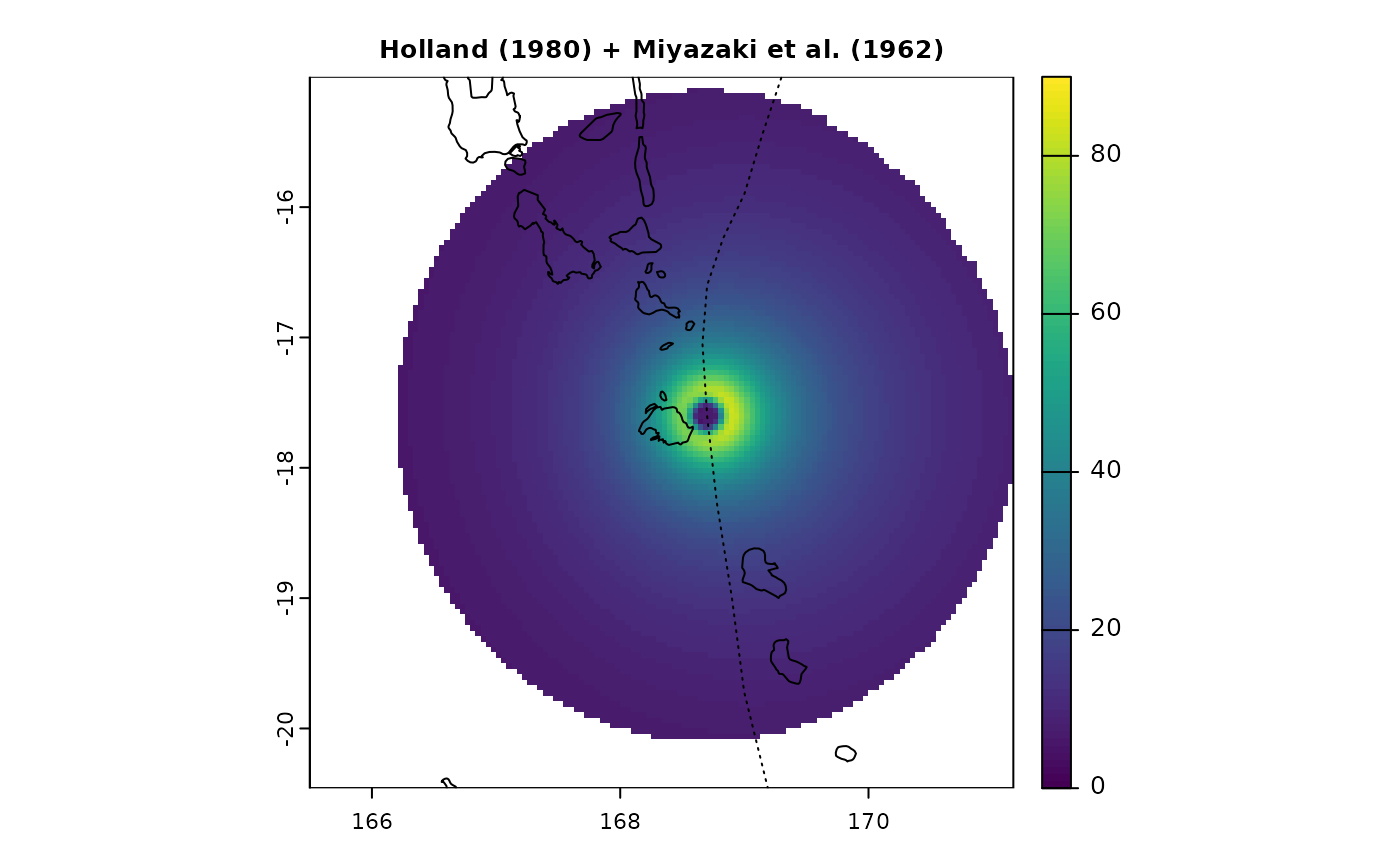

pf <- spatialBehaviour(st, product = "Profiles", method = "Willoughby", asymmetry = "Miyazaki", verbose = 0)
terra::plot(pf$PAM_Speed_41, main = "Willoughby et al. (2006) + Miyazaki et al. (1962)", cex.main = 0.8, range = c(0, 90))
terra::plot(countriesHigh, add = TRUE)
lines(PAM$lon, PAM$lat, lty = 3)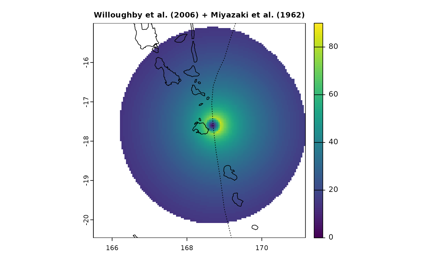

pf <- spatialBehaviour(st, product = "Profiles", method = "Holland", asymmetry = "Chen", verbose = 0)
terra::plot(pf$PAM_Speed_41, main = "Holland (1980) + Chen (1994)", cex.main = 0.8, range = c(0, 90))
terra::plot(countriesHigh, add = TRUE)
lines(PAM$lon, PAM$lat, lty = 3)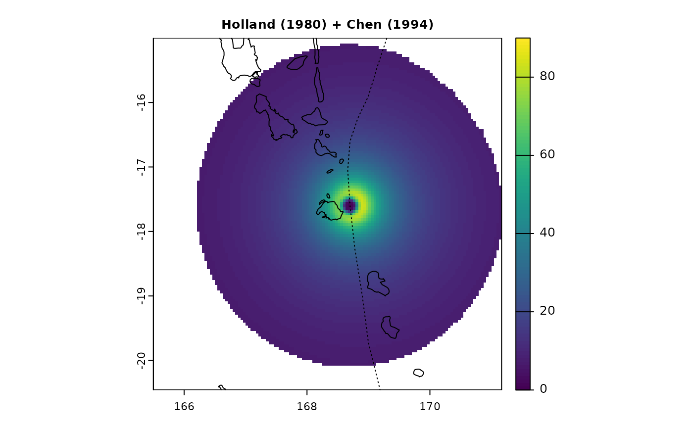

pf <- spatialBehaviour(st, product = "Profiles", method = "Willoughby", asymmetry = "Chen", verbose = 0)
terra::plot(pf$PAM_Speed_41, main = "Willoughby et al. (2006) + Chen (1994)", cex.main = 0.8, range = c(0, 90))
terra::plot(countriesHigh, add = TRUE)
lines(PAM$lon, PAM$lat, lty = 3)

pf <- spatialBehaviour(st, product = "Profiles", method = "Boose", verbose = 0)
terra::plot(pf$PAM_Speed_41, main = "Boose et al. (2004)", cex.main = 0.8, range = c(0, 90))
terra::plot(countriesHigh, add = TRUE)
lines(PAM$lon, PAM$lat, lty = 3)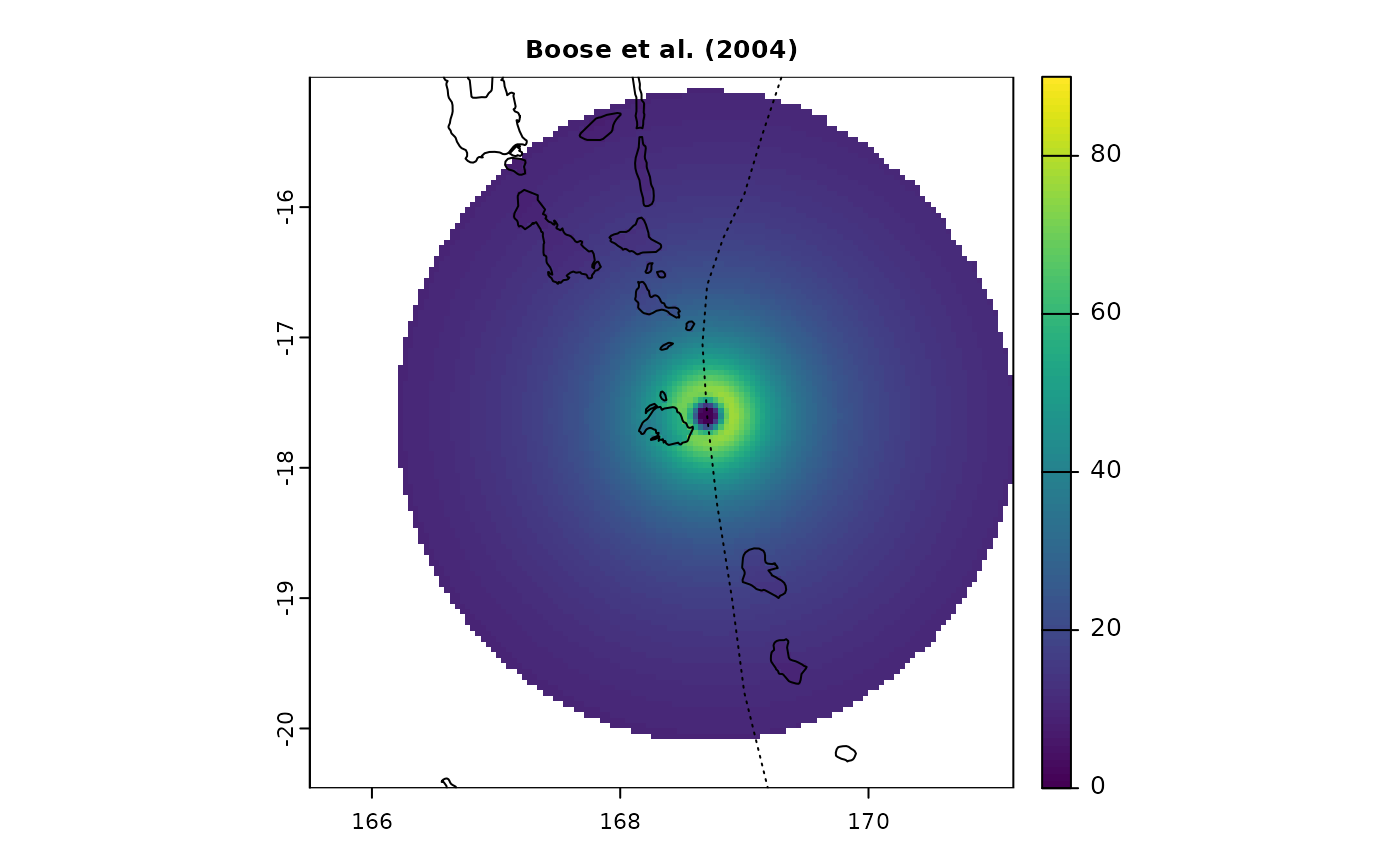

par(oldpar)

References

Boose, E. R., Kristen E. Chamberlin, and David R. Foster. 2001. “Landscape and Regional Impacts of Hurricanes in New England.” Ecological Monographs 71 (1): 27–48. https://doi.org/10.1890/0012-9615(2001)071[0027:LARIOH]2.0.CO;2.

Boose, E. R., Mayra I. Serrano, and David R. Foster. 2004. “Landscape and Regional Impacts of Hurricanes in Puerto Rico.” Ecological Monographs 74 (2): 335–52. https://doi.org/10.1890/02-4057.

Chen, KM. 1994. “A Computation Method for Typhoon Wind Field.” Tropic Oceanology 13 (2): 41–48.

Holland, Greg J. 1980. “An Analytic Model of the Wind and Pressure Profiles in Hurricanes.” Monthly Weather Review 108 (8): 1212–18. https://doi.org/10.1175/1520-0493(1980)108<1212:AAMOTW>2.0.CO;2.

Miyazaki, M., T. Ueno, and S. Unoki. 1962. “The Theoretical Investigations of Typhoon Surges Along the Japanese Coast (II).” Oceanographical Magazine 13 (2): 103–17. https://cir.nii.ac.jp/crid/1573105975206118656.

Willoughby, H. E. 1995. “Normal-Mode Initialization of Barotropic Vortex Motion Models.” Journal of the Atmospheric Sciences 52 (24): 4501–14. https://doi.org/10.1175/1520-0469(1995)052<4501:NMIOBV>2.0.CO;2.

Willoughby, H. E., R. W. R. Darling, and M. E. Rahn. 2006. “Parametric Representation of the Primary Hurricane Vortex. Part II: A New Family of Sectionally Continuous Profiles.” Monthly Weather Review 134 (4): 1102–20. https://doi.org/10.1175/MWR3106.1.

Willoughby, H. E., and M. E. Rahn. 2004. “Parametric Representation of the Primary Hurricane Vortex. Part I: Observations and Evaluation of the Holland (1980) Model.” Monthly Weather Review 132 (12): 3033–48. https://doi.org/10.1175/MWR2831.1.