Extract Storms

The defStormsList() function allows to extract tropical cyclone track data for a given tropical cyclone or set of tropical cyclones nearby a given location of interest (loi). The loi can be defined using a country name, a specific point (defined by its longitude and latitude coordinates), or any user imported or defined spatial polygon shapefiles. By default only observations located within 300 km around the loi are extracted but this can be changed using the max_dist argument. Users can also extract tropical cyclones using the name of the storm or the season during which it occurred. If both the name and the season arguments are not filled then the defStormsList() function extracts all tropical cyclones since the first cyclonic season in the database. Once the data are extracted, the plotStorms() function can be used to visualize the trajectories and points of observation of extracted tropical cyclones on a map.

In the following example we use the test_dataset provided with the package to illustrate how cyclone track data can be extracted and visualised using country and cyclone names, specific point locations, and polygon shapefiles, as described below.

Getting and ploting tropical cyclone track data

Using country names

We extract data on the tropical cyclone Pam (2015) nearby Vanuatu as follows:

sds <- defStormsDataset(verbose = 0)

## Warning in checkInputsdefStormsDataset(filename, sep, fields, basin, seasons, : No basin argument specified. StormR will work as expected
##              but cannot use basin filtering for speed-up when collecting data

st <- defStormsList(sds = sds, loi = "Vanuatu", names = "PAM", verbose = 0)

The defStormsList() function returns a stormsList object in which the first slot @data contains a list of Storm objects. With the above specification the stormsList contains only one Storm object corresponding to cyclone PAM and the track data can be obtained using the getObs() function as follows:

head(getObs(st, name = "PAM"))

##              iso.time      lon       lat msw scale rmw   pres   poci
## 1 2015-03-08 12:00:00 168.9000 -7.500000  13     0  93 100400 100500
## 2 2015-03-08 15:00:00 169.0425 -7.652509  14     0  93 100200 100200
## 3 2015-03-08 18:00:00 169.2000 -7.800000  15     0  93 100000 100000
## 4 2015-03-08 21:00:00 169.3850 -7.942489  15     0  93 100000 100000
## 5 2015-03-09 00:00:00 169.6000 -8.100000  15     0  93 100000 100100
## 6 2015-03-09 03:00:00 169.8425 -8.284999  16     0  93  99800 100100

The number of observation and the indices of the observations can be obtained using the getNbObs() and getInObs() as follows:

getNbObs(st, name = "PAM")

## [1] 57

getInObs(st, name = "PAM")

##  [1] 28 29 30 31 32 33 34 35 36 37 38 39 40 41 42 43 44 45 46 47

The data can be visualised on a map as follows:

plotStorms(st, labels = TRUE)

Using a specified point location

We can extract all tropical cyclones near Nouméa (longitude = 166.45, latitude = -22.27) between 2015 and 2021 as follows:

pt <- c(166.45, -22.27)
st <- defStormsList(sds = sds, loi = pt, seasons = c(2015, 2021), verbose = 0)

The number, the names, and the season of occurrence of the storms in the returned stormsList object can be obtained using the getNbStorms(), getNames(), and getSeasons() functions as follows:

getNbStorms(st)

## [1] 4

getNames(st)

## [1] "SOLO"   "GRETEL" "LUCAS"  "NIRAN"

getSeasons(st)

##   SOLO GRETEL  LUCAS  NIRAN 
##   2015   2020   2021   2021

We can plot track data for the topical cyclone Niran only using the names argument of the plotStorms() function as follows:

plotStorms(st, names = "NIRAN", labels = TRUE, legends = "bottomleft")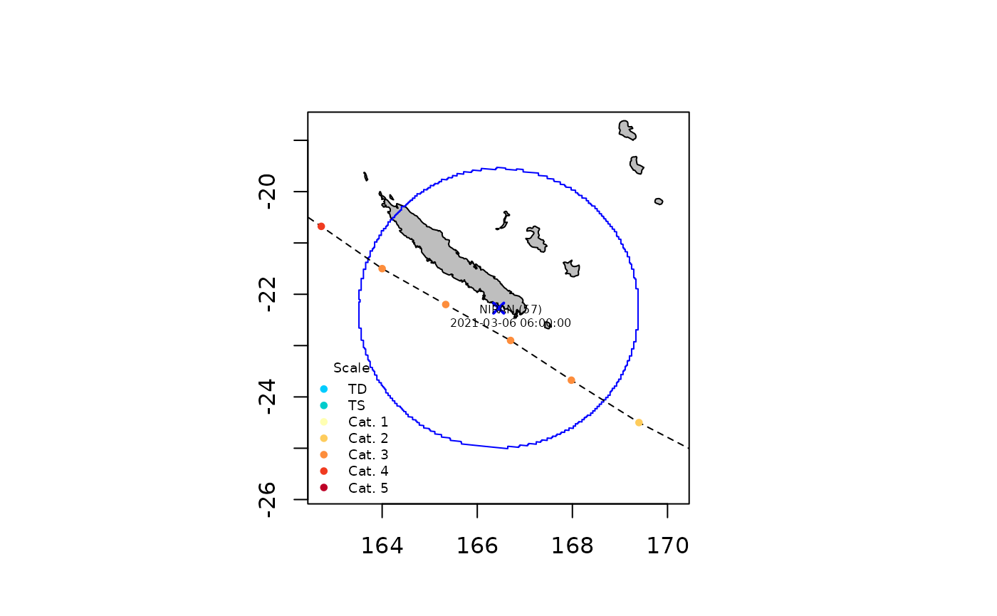

The track data for Niran can also be extracted and stored in a new object using the getStorm() function as follows:

NIRAN <- getStorm(st, name = "NIRAN")
getNames(NIRAN)

## [1] "NIRAN"

Using a user defined spatial polygon shapefile

We can extract all tropical cyclones that occurred between 2015 and 2021 near the New Caledonia exclusive economic zone using the eezNC shapefile provided with the StormR package as follows:

sp <- eezNC
st <- defStormsList(sds = sds, loi = eezNC, season = c(2015, 2021), verbose = 0)

Information about the spatial extent of the track data exaction can be obtained using the getLOI(), getBuffer(), and getBufferSize() functions as follows:

LOI <- getLOI(st)
Buffer <- getBuffer(st)
BufferSize <- getBufferSize(st)
terra::plot(Buffer, lty = 3, main = paste(BufferSize, "km buffer arround New Caledonian EEZ", sep = " "))
terra::plot(LOI, add = TRUE)
terra::plot(countriesHigh, add = TRUE)

Using different wind scale

By default the Saffir-Simpson hurricane wind scale (SSHS) is used in defStormsList() to assign level to storms.

The maximum level reached in the scale for each cyclone can then be obtained using the getScale() function as follows:

getScale(st)

##     PAM    SOLO     ULA WINSTON    ZENA    UESI  GRETEL   LUCAS   NIRAN 
##       6       1       5       6       3       2       2       2       6

In this case, the SSHS scale is composed of 6 thresholds resulting in 6 levels spanning from level 0 to level 6.

We can only plot cyclones that reached level 5 and 6 using the category argument of the plotStorms() function as follows:

plotStorms(st, category = c(5, 6), labels = FALSE, legends = "topright")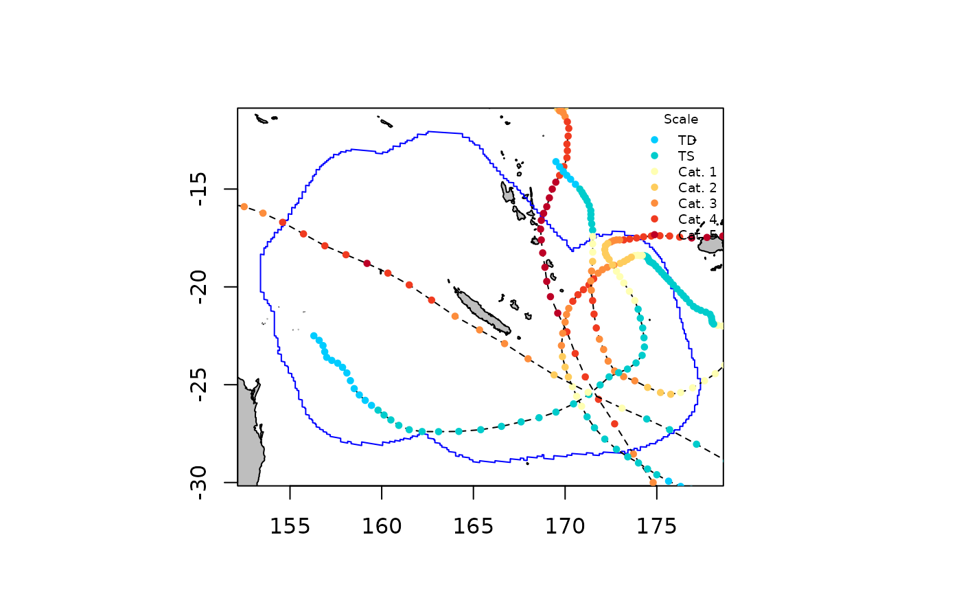

Finally, the user can choose his own scale and associated palette, by setting the scale and scalePalette inputs in defStormsList(). In the following example, we use the Tokyo’s tropical cyclone intensity scale to analyse tropical storm PAM.

StormR provides default palette and category names:

# Tokyo's tropical cyclone intensity scale
RSMCScale <- c(16.94, 24.44, 32.5, 43.33, 53.61)

sts_jpn <- defStormsList(sds = sds,
                         loi = "Vanuatu",
                         names = "PAM",
                         scale = RSMCScale,
                         verbose = 0)

plotStorms(sts_jpn)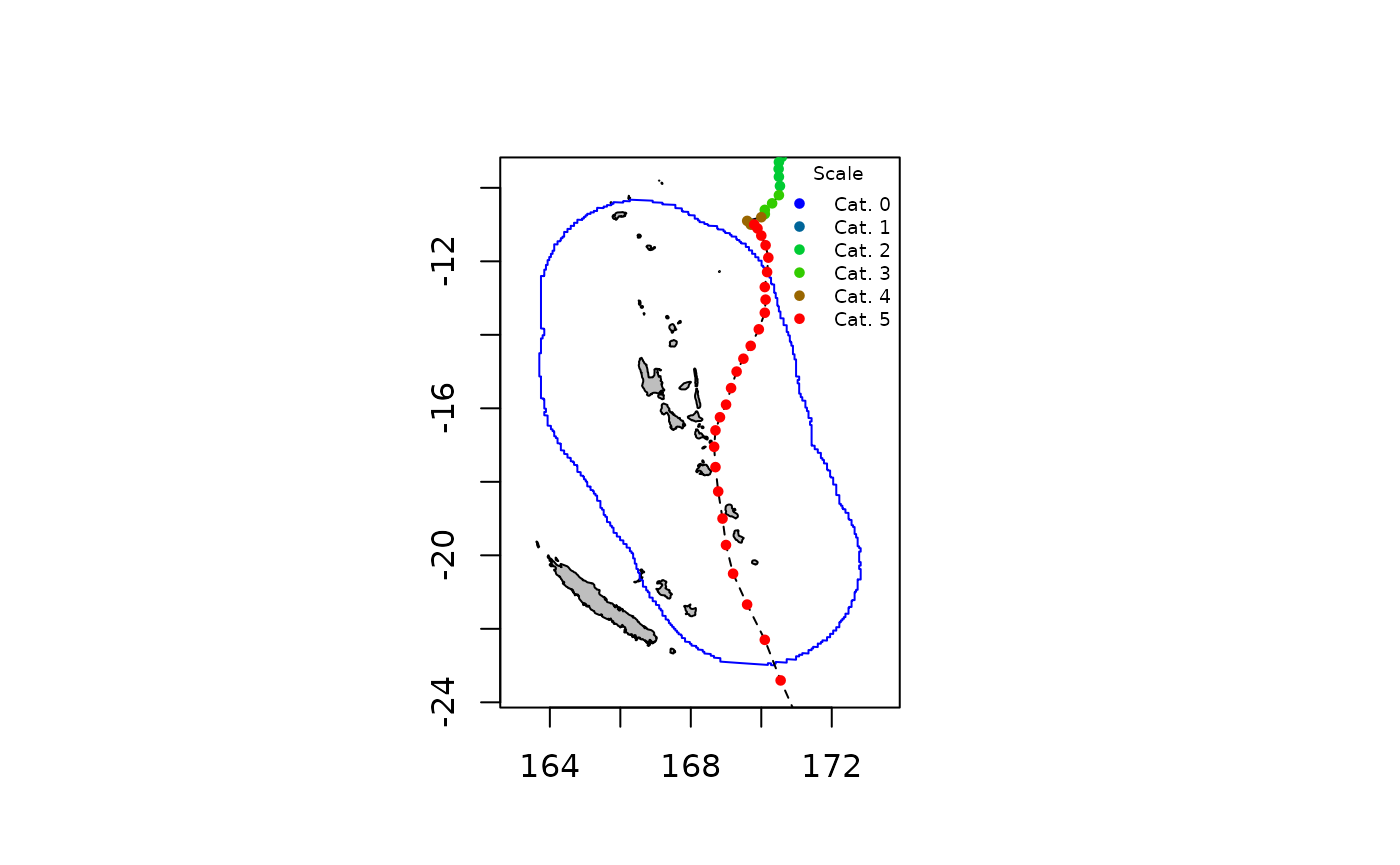

But you can also easily customize them:

RSMCPalette <- c("#6ec1ea", "#4dffff", "#c0ffc0", "#ffd98c", "#ff738a", "#a188fc")
names(RSMCPalette) <- c("Tropical depression",
                        "Tropical storm",
                        "Severe tropical storm",
                        "Typhoon",
                        "Very strong typhoon",
                        "Violent typhoon")

sts_jpn <- defStormsList(sds = sds,
                         loi = "Vanuatu",
                         names = "PAM",
                         scale = RSMCScale,
                         scalePalette = RSMCPalette,
                         verbose = 0)

plotStorms(sts_jpn)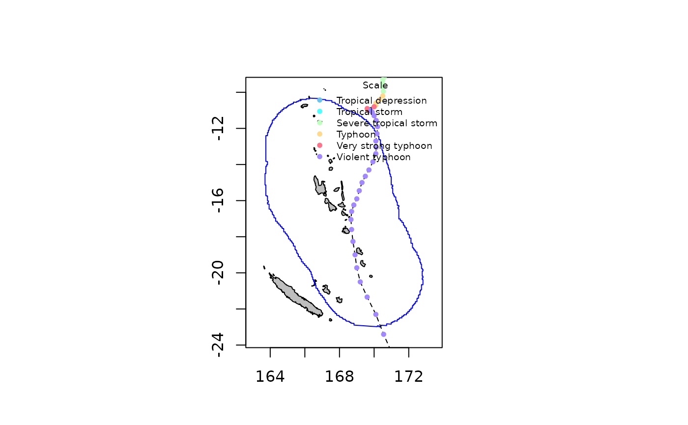

Dynamic plot

plotStorms allows the user to dynamically plot tracks within an interactive map using leaflet library by setting dynamicPlot to TRUE. Doing so, the user can explore the map the way he wants and click and each dotted colored observations to see there informations.