Using the Plot Query App and query_plots()
using-query-plots.RmdOverview
CafriplotsR offers two complementary ways to access forest plot data:
-
Interactive Shiny app
(
launch_query_plots_app()) — point-and-click interface with live map, plot selection, and download -
R function (
query_plots()) — reproducible, scriptable access for automated workflows
A key bridge between the two is the “Equivalent R
Code” panel in the app, which shows the exact
query_plots() call that reproduces what you configured
interactively.
Part 1 — Interactive Shiny App
Launching the App
# Launch with default language (French)
launch_query_plots_app()

# Launch in English
launch_query_plots_app(language = "en")

# Launch in browser on a specific port
launch_query_plots_app(language = "en", launch.browser = TRUE, port = 8080)

# Reuse an existing connection pool (avoids repeated login prompts)
pool <- create_pool_main()
launch_query_plots_app(pool_main = pool)
The app will prompt for database credentials if no pool is provided.
Use setup_db_credentials() to store credentials in
~/.Renviron to skip the prompt on future sessions.
App Overview
The app has four tabs accessible from the top navigation bar:
| Tab | Purpose |
|---|---|
| Query Builder | Define filters and execute the metadata query |
| Results & Extraction | Map, table, plot selection, extraction config, download |
| Statistics | Summary statistics and charts for extracted data |
| About | App documentation and package information |
The language toggle (EN / FR) is always visible in the top-right corner. The switch is instant and affects all UI elements.
Screenshot to add: full app view after login, showing the four-tab navigation bar (
app-query-nav-tabs.png).
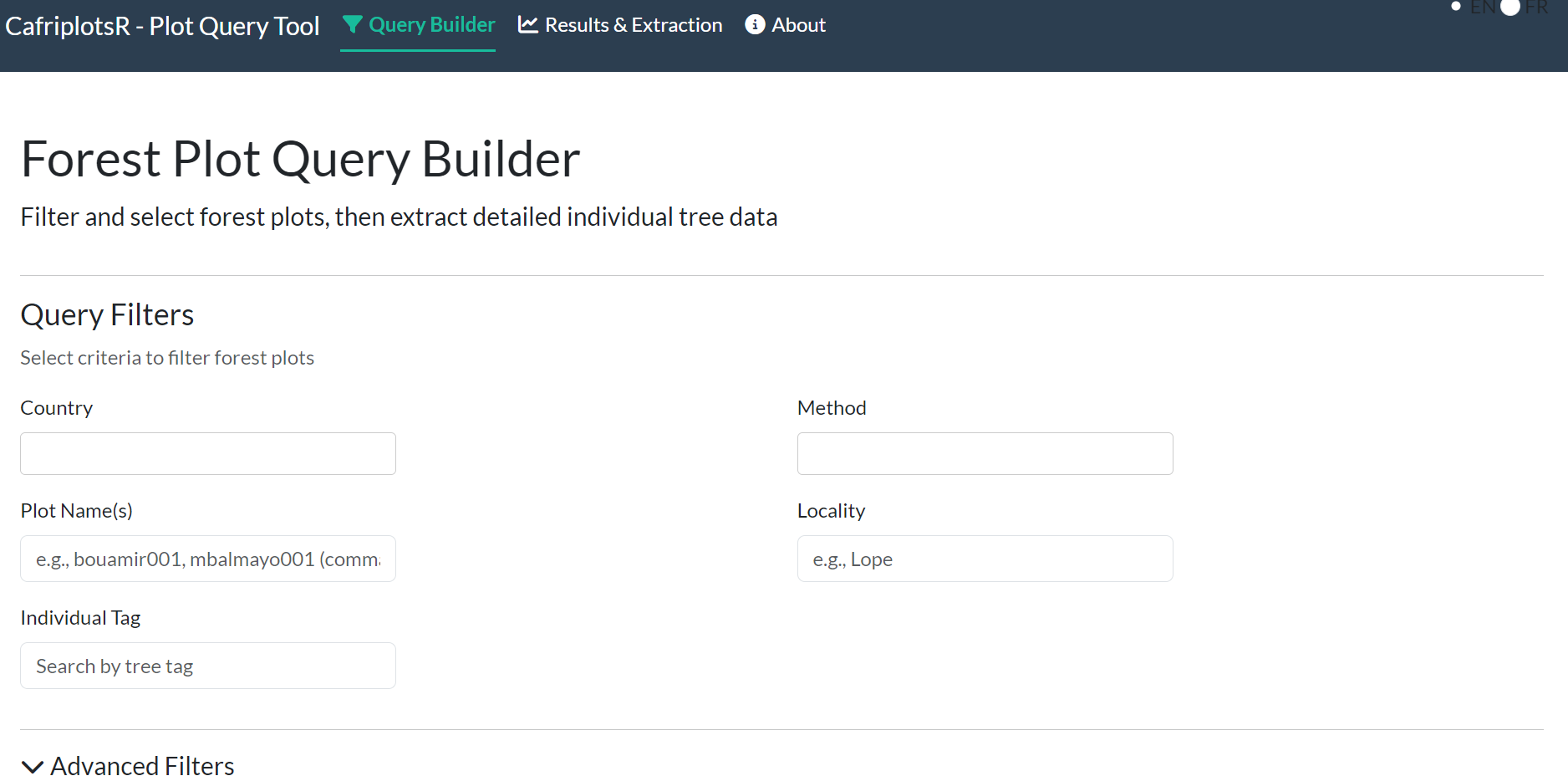
Tab 1 — Query Builder
Basic Filters
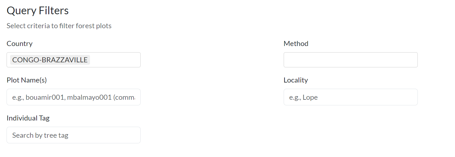
- Country — multi-select dropdown of available countries
- Method — inventory method (e.g., “1 ha plot”, “Long Transect”)
- Plot Name(s) — partial or exact text search; comma-separate multiple names
- Locality — search by locality name
- Individual Tag — search by tree tag number
Advanced Filters
Click Advanced Filters to expand additional options:
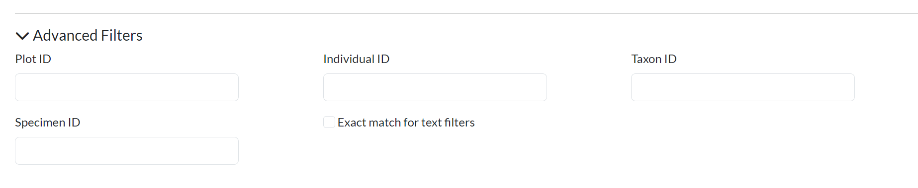
- Plot ID — search by internal database plot ID
- Individual ID — search by specific individual ID
- Taxon ID — filter by taxonomic ID
- Specimen ID — search by herbarium specimen ID
- Exact match — toggle for strict text matching (default: partial)
Tab 2 — Results & Extraction
This tab has five stacked sections that guide you from visualising results to downloading data.
Section A — Interactive Map
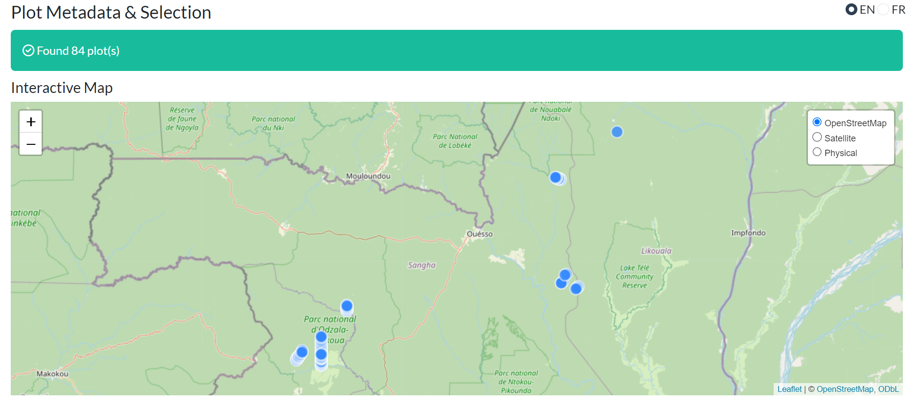
- Basemap layers — OpenStreetMap, Satellite, Physical
- Clickable markers — show plot name, country, method, area
- Map and table are synchronised: selecting rows in the table highlights the corresponding markers
Section B — Metadata Table
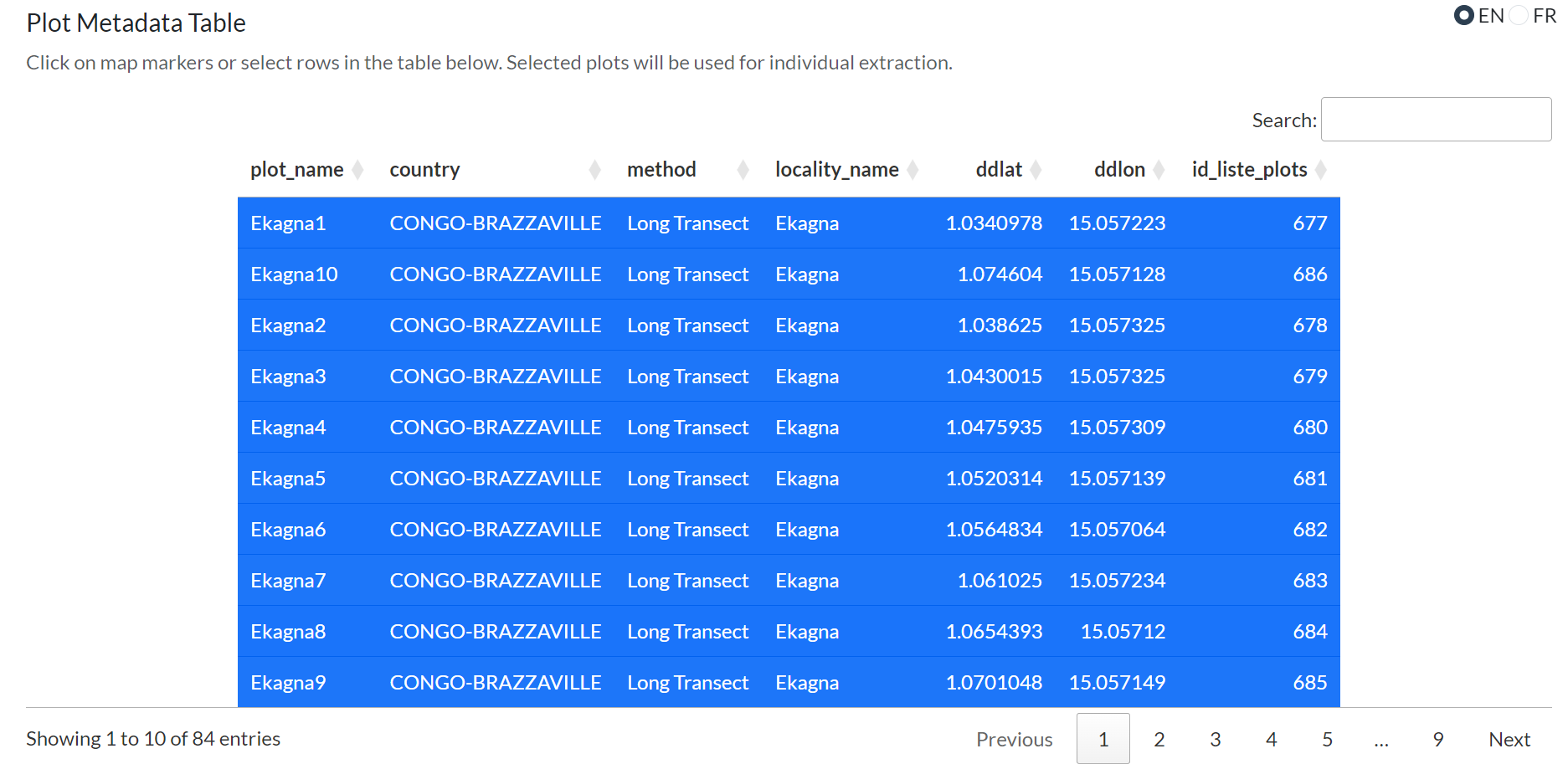
A sortable, searchable table of all plot metadata returned by the query. Click column headers to sort; use the search box to filter rows.
Section C — Plot Selection
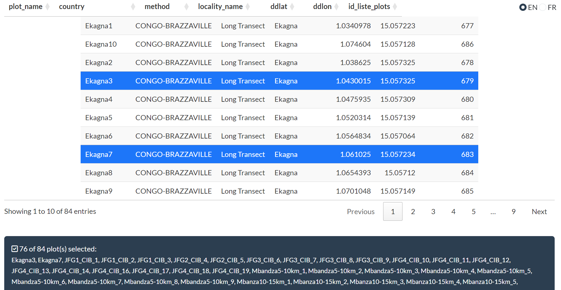
Click rows to select or deselect individual plots. A counter shows the number of selected plots. All plots are pre-selected by default.
Section D — Extraction Configuration
After selecting plots, configure how individual tree data should be extracted:
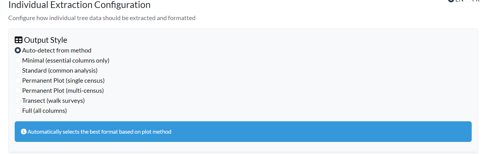
Output Style — controls which columns and tables are returned:
| Style | Best for |
|---|---|
| Auto-detect | Let the app choose based on the plot method |
| Minimal | Quick exploration — essential columns only |
| Standard | General ecological analysis |
| Permanent Plot | Single-census permanent plot monitoring |
| Permanent Plot (multi-census) | Time-series format with _census_N columns |
| Transect | Walk survey format |
| Full | Complete dataset, all columns |
Census Handling:

- Census Strategy — Last (default), First, or Mean across censuses
-
Show multiple census data — creates
dbh_census_1,dbh_census_2, … columns; automatically selects the Permanent Plot (multi-census) style -
Individual features format:
- Wide (default) — one row per individual, traits as columns; values are aggregated when multiple measurements exist for the same individual
-
Long — one row per measurement; includes
trait,traitvalue,census_name, andcensus_datecolumns - Census pairs — one row per consecutive pair of censuses per individual; useful for computing growth rates
Data Organisation:
- Concatenate multiple stems — combine multi-stemmed tree measurements
- Remove database IDs — hide internal ID columns for cleaner output
- Issues handling — remove, include, or ignore flagged records
- Include issue flags — add quality flag columns to the output
Note:
"long"and"census pairs"formats are incompatible with Concatenate multiple stems; that option is automatically disabled when either long-format mode is selected.
Additional Data:
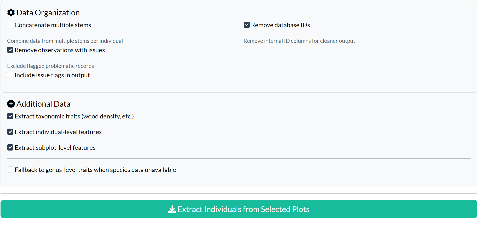
- Extract taxonomic traits — wood density, growth form, etc.
- Extract individual-level features — tree-specific measurements
- Extract subplot-level features — subplot characteristics
- Fallback to genus-level traits — use genus data when species traits are unavailable
Click Extract Individuals from Selected Plots to run the extraction.
Section E — Results Display and Download
Results are organised in tabs: Individuals, Metadata, Censuses, Height-Diameter (when applicable), and Column Documentation.
Screenshot to add: results display showing the result tabs after extraction, with the Column Documentation tab visible (
app-query-results-display.png).
The Column Documentation tab is always present after extraction. It contains a searchable table describing every output column: its original database name, a plain-language description, category, unit, and any contextual notes. This is the fastest way to understand what each column means without consulting external documentation.
The column documentation table is also exportable: select it via the download checkboxes to include it as an additional sheet in Excel exports, a separate CSV in the ZIP archive, or an element of the RDS list.
Download your data using the download panel:
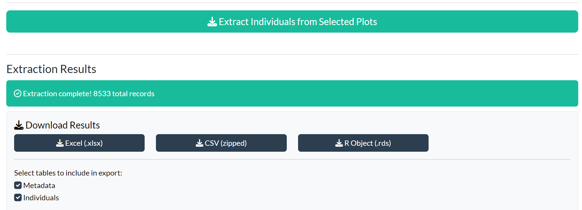
| Format | Notes |
|---|---|
| Excel (.xlsx) | Multi-sheet workbook, one sheet per table |
| CSV (zipped) | Separate CSV files in a ZIP archive |
| R Object (.rds) | Native R format; preserves list structure and data types |
| Shapefile (.zip) | Spatial data (requires coordinate columns) |
Use the checkboxes to select which tables to include before downloading.
Section F — Equivalent R Code
After running a query or extraction, the Equivalent R
Code panel shows the exact query_plots() calls
that reproduce your results:
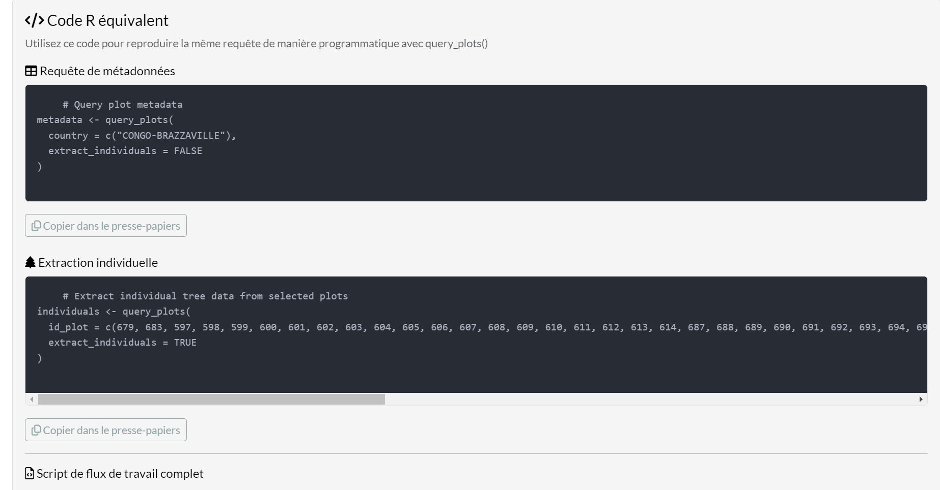
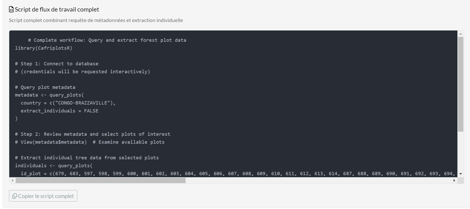
Three code sections are provided:
- Metadata Query — filter and retrieve plot metadata
- Individual Extraction — extract tree data with your chosen options
- Complete Workflow Script — both steps in a single ready-to-run script
Click Copy to clipboard to copy any section directly into your R editor.
Tab 3 — Statistics
The Statistics tab displays summary cards and charts that update automatically once individual data has been extracted:
- Total number of plots extracted
- Total number of individuals (stems)
- Number of species
- Number of families
- Diameter distribution histogram (when DBH data are available)
Screenshot to add: Statistics tab showing the four summary cards and the diameter histogram (
app-query-statistics.png).
Tab 4 — About
The About tab contains a description of the app’s features and package metadata (version, authors, links to documentation and repository).
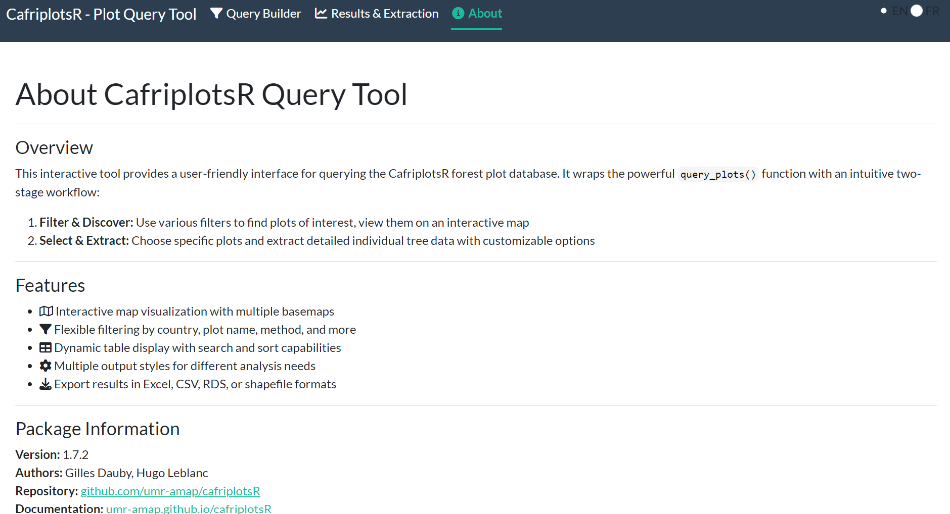
Screenshot to update: the About page now shows version 1.7.2 and the updated authors list — retake if your existing screenshot is from an older version.
From App to Script
The typical workflow is:
- Use the app to explore plots and configure options interactively
- Copy the generated code from the Equivalent R Code panel
- Paste it into your analysis script for reproducible, automated runs
# Example code generated by the app after selecting Cameroon 1-ha plots

# Step 1: query metadata
metadata <- query_plots(
  country = "Cameroon",
  method = "1 ha plot",
  extract_individuals = FALSE
)

# Step 2: extract individuals from selected plots
result <- query_plots(
  id_plot = c(1, 5, 12),
  extract_individuals = TRUE,
  output_style = "permanent_plot",
  extract_traits = TRUE,
  census_strategy = "last"
)
App vs. Function: When to Use Each
| Use case | Recommendation |
|---|---|
| First exploration, unknown plot IDs | App |
| Interactive map selection | App |
| Learning function parameters | App — copy generated code |
| Reproducible analysis scripts | query_plots() |
| Automated data pipelines | query_plots() |
| Batch processing many queries | query_plots() |
Part 2 — query_plots() Function
Database Connection
# Recommended: interactive credential prompt
mydb <- call.mydb()

# Use credentials stored in ~/.Renviron
mydb <- call.mydb(use_env_credentials = TRUE)
The taxa database connection is created automatically inside
query_plots() when needed. Supply it explicitly via
con.taxa to reuse an existing connection and avoid repeated
prompts:
mydb      <- call.mydb()
mydb_taxa <- call.mydb.taxa()

result <- query_plots(
  plot_name = "mbalmayo001",
  extract_individuals = TRUE,
  con      = mydb,
  con.taxa = mydb_taxa
)
Basic Usage
Metadata only (no tree data)
plots <- query_plots(
  plot_name = "mbalmayo001",
  extract_individuals = FALSE
)
plots$metadata
Including individual trees
result <- query_plots(
  plot_name = "mbalmayo001",
  extract_individuals = TRUE
)

names(result)       # e.g. metadata, individuals, censuses, height_diameter
result$individuals  # one row per stem
result$censuses     # census dates and team information
Output Styles
query_plots() always returns a named
list. The tables included and the columns kept depend on
output_style. Built-in styles:
output_style |
Description | Additional tables |
|---|---|---|
"auto" |
Detected from plot method (default) |
varies |
"minimal" |
Essential plot metadata only | — |
"standard" |
General-purpose output for analysis | — |
"permanent_plot" |
Permanent plot monitoring, single/most-recent census |
censuses, height_diameter
|
"permanent_plot_multi_census" |
Multi-census wide format (_census_N columns) |
censuses, height_diameter
|
"transect" |
Simplified output for transect / walk surveys | — |
"census_pairs" |
One row per consecutive census pair per individual | — |
"full" |
Keep every metadata and individual column | — |
# Auto-detect from method (recommended)
result_auto <- query_plots(
  plot_name = "mbalmayo001",
  extract_individuals = TRUE
)

# Force a specific style
result_perm <- query_plots(
  plot_name = "mbalmayo001",
  extract_individuals = TRUE,
  output_style = "permanent_plot"
)

# Full output keeps every column on the metadata and individuals tables
result_full <- query_plots(
  plot_name = "mbalmayo001",
  extract_individuals = TRUE,
  output_style = "full"
)
names(result_full$individuals)
Inspecting built-in styles
Two helper functions let you discover what each style does without leaving R:
# Summary table of all built-in styles
list_output_styles()

# Full configuration of a single style, with a pretty print method
get_output_style("permanent_plot")

# Drop the class to access fields programmatically
cfg <- unclass(get_output_style("permanent_plot"))
cfg$metadata_columns
cfg$remove_patterns
list_output_styles() returns a tibble with one row per
style and counts of explicit columns / regex patterns.
get_output_style() returns a plot_output_style
object whose print method groups fields by purpose (column selection,
regex filters, renames, additional tables, flags).
Custom output styles
If none of the built-in styles fits, build your own with
output_style() and pass the resulting object straight to
query_plots():
my_style <- output_style(
  description         = "Just IDs and species",
  metadata_columns    = c("plot_name", "country", "id_liste_plots"),
  individuals_columns = c("id_n", "tag", "tax_fam", "tax_gen", "tax_sp_level")
)

result <- query_plots(
  plot_name           = "mbalmayo001",
  extract_individuals = TRUE,
  output_style        = my_style
)
Use based_on to start from an existing style and
override only the fields you want to change. Override semantics
are “replace, not append”: any field you pass replaces the
parent’s value entirely. To clear a vector field while inheriting the
rest, pass an empty vector (remove_patterns = character());
to inherit unchanged, leave it unspecified.
# Start from permanent_plot, but drop all trait_* columns from the output
perm_no_traits <- output_style(
  based_on        = "permanent_plot",
  remove_patterns = c(
    "^id_(?!n|liste_plots)", "^date_modif",
    "_census_\\d+$", "^trait_"
  )
)
perm_no_traits   # pretty-printed summary

result <- query_plots(
  plot_name           = "mbalmayo001",
  extract_individuals = TRUE,
  output_style        = perm_no_traits
)
Custom style objects live only in the current R session. To reuse
one, assign it to a variable, save it with saveRDS(), or
put the constructor call in your .Rprofile / a project
script.
keep_patterns and remove_patterns
Beyond the explicit metadata_columns /
individuals_columns lists, every style supports two
regex-based filters applied on top of the column selection:
-
keep_patterns— Perl-compatible regexes. Any column whose name matches any pattern is added to the keep list (useful for grabbing whole groups of feature columns like^feat_orwood_density). -
remove_patterns— applied afterkeep_patternsto drop columns. Often used to remove internal IDs ("^id_(?!n|liste_plots)"), modification timestamps ("^date_modif"), or per-census suffix columns ("_census_\\d+$").
# Keep every wood density and stem diameter column, drop internal IDs
my_style <- output_style(
  based_on        = "standard",
  keep_patterns   = c("wood_density", "stem_diameter"),
  remove_patterns = c("^id_(?!n|liste_plots)", "^date_modif")
)
Filtering Options
# By country
query_plots(country = "Cameroon", extract_individuals = FALSE)

# By method
query_plots(method = "1 ha plot", extract_individuals = FALSE)

# Multiple countries or methods
query_plots(country = c("Cameroon", "Gabon"), extract_individuals = FALSE)

# By locality
query_plots(locality_name = "Dja", extract_individuals = FALSE)

# By plot ID (most efficient when IDs are already known)
query_plots(id_plot = c(1, 2, 3), extract_individuals = TRUE)

# By individual tag (implies extract_individuals = TRUE)
query_plots(plot_name = "mbalmayo001", tag = "1234")

# By taxon ID
query_plots(plot_name = "mbalmayo001", id_tax = 115, extract_individuals = TRUE)

# By herbarium specimen ID
query_plots(id_specimen = 42, extract_individuals = TRUE)

# Exact plot name match (default is partial)
query_plots(plot_name = "mbalmayo001", exact_match = TRUE, extract_individuals = FALSE)
Handling Multiple Censuses
# Last census only (default)
last <- query_plots(
  plot_name = "mbalmayo",
  extract_individuals = TRUE,
  census_strategy = "last"
)

# First census
first <- query_plots(
  plot_name = "mbalmayo",
  extract_individuals = TRUE,
  census_strategy = "first"
)

# Mean values across all censuses
averaged <- query_plots(
  plot_name = "mbalmayo",
  extract_individuals = TRUE,
  census_strategy = "mean"
)

# All censuses as separate columns (dbh_census_1, dbh_census_2, …)
multi <- query_plots(
  plot_name = "mbalmayo",
  extract_individuals = TRUE,
  show_multiple_census = TRUE   # automatically uses permanent_plot_multi_census style
)
multi$censuses   # census dates
head(multi$individuals)
Individual Features Format
Three row structures are available:
# Wide (default): one row per individual, traits as columns
wide <- query_plots(
  plot_name = "mbalmayo001",
  extract_individuals = TRUE,
  individual_features_format = "wide"
)
# Long: one row per measurement
long <- query_plots(
  plot_name = "mbalmayo001",
  extract_individuals = TRUE,
  individual_features_format = "long"
)
# Extra columns: trait, traitvalue, traitvalue_char, valuetype, census_name, census_date
long$individuals |>
  dplyr::select(plot_name, tag, tax_sp_level, trait, traitvalue, census_name, census_date)
# Census pairs: one row per consecutive census pair per individual
# Useful for computing diameter growth between censuses
pairs <- query_plots(
  plot_name = "mbalmayo",
  extract_individuals = TRUE,
  individual_features_format = "census_pairs"
)
# Output style is automatically set to "census_pairs"
Taxonomic Backbone
# Internal taxonomy (default)
result_internal <- query_plots(
  plot_name = "mbalmayo001",
  extract_individuals = TRUE,
  backbone = "internal"
)

# WCVP (World Checklist of Vascular Plants)
result_wcvp <- query_plots(
  plot_name = "mbalmayo001",
  extract_individuals = TRUE,
  backbone = "wcvp"
)
Additional Data Options
result <- query_plots(
  plot_name = "mbalmayo001",
  extract_individuals = TRUE,
  extract_traits            = TRUE,   # taxonomic traits (wood density, growth form …)
  extract_individual_features = TRUE, # tree-level measurements
  extract_subplot_features  = TRUE,   # subplot characteristics
  traits_to_genera          = FALSE,  # fall back to genus-level when species traits absent
  wd_fam_level              = FALSE,  # fall back to family-level wood density
  include_liana             = FALSE   # set TRUE to keep lianas in the output
)
Spatial Data
# Default: one representative coordinate per plot
plots <- query_plots(country = "Gabon", extract_individuals = FALSE)
plots$metadata[, c("plot_name", "latitude", "longitude")]

# All coordinate points (corners, subplot centres …)
all_coords <- query_plots(
  plot_name = "mbalmayo",
  extract_individuals   = FALSE,
  extract_coordinates   = TRUE   # replaces deprecated show_all_coordinates
)
all_coords$coordinates_sf        # sf object
Note:
show_all_coordinateswas deprecated in v1.9.4. Useextract_coordinatesinstead.
# Display an interactive Leaflet map (opens in the RStudio Viewer)
query_plots(country = "Cameroon", extract_individuals = FALSE, map = TRUE)
Keeping Database IDs
result <- query_plots(
  plot_name = "mbalmayo001",
  extract_individuals = TRUE,
  remove_ids   = FALSE,
  output_style = "full"
)
names(result$extract)  # includes id_liste_plots, id_census, id_n …
Handling Data Quality Issues
# Remove flagged records (default)
clean <- query_plots(
  plot_name = "mbalmayo001", extract_individuals = TRUE,
  issues = "remove"
)

# Include all records regardless of flags
all_records <- query_plots(
  plot_name = "mbalmayo001", extract_individuals = TRUE,
  issues = "include"
)

# Keep flagged records but add quality flag columns
with_flags <- query_plots(
  plot_name = "mbalmayo001", extract_individuals = TRUE,
  issues = "ignore"
)
Complex Query Example
result <- query_plots(
  country      = "Cameroon",
  locality_name = "Dja",
  method       = "1 ha plot",
  extract_individuals         = TRUE,
  extract_traits              = TRUE,
  extract_individual_features = TRUE,
  show_multiple_census        = TRUE,
  extract_coordinates         = TRUE,
  remove_ids                  = FALSE,
  output_style                = "permanent_plot_multi_census"
)

names(result)
Performance Tips
- Start with
extract_individuals = FALSEto explore metadata before pulling tree data - Filter by
id_plotwhen plot IDs are already known — it is the most efficient route - Enable
extract_traitsandextract_individual_featuresonly when needed - Choose the most specific
output_styleto avoid loading unused columns
Troubleshooting
# Check connection status
print_connection_status()

# Run a full connection diagnostic
db_diagnostic()

# Close all connections and clear cached credentials
cleanup_connections()
Row-level security is enforced on the database: you can only access plots and individuals that your database account has permission to view.