computeTEW

The computeTEW() function allows computing topographic exposure to wind (TEW) Boose et al. (1994) for each cell of a regular grid (i.e., a raster) for a given tropical cyclone or set of tropical cyclones. The product="TEW1wd" and product="TEW" argument allows producing exposure fields during the lifespan of the cyclone. The computeTEW() function also allows to compute three associated summary statistics: the maximum and mean TEW for each cell during the cyclone (product="TEW1wdMax" and product="TEW1wdMean", respectively) and the TEW computed for each pixel with the direction at maximal sustained speed along the cyclone (product="TEWIntegrated").

Then the plotTEW() and the writeRast() functions can be used to visualize and export the output.

In the following example we use the test_dataset and test_datadtm provided with the package to illustrate how cyclone track data can be used to compute, plot, and export topographic exposure profiles or summary statistics.

Computing and plotting computeTEW products

Exctracting storm

We can compute the behaviour of winds generated by the topical cyclone Pam (2015) near Vanuatu. First, track data are extracted as follows:

sds <- defStormsDataset()

## Warning: No basin argument specified. StormR will work as expected
##              but cannot use basin filtering for speed-up when collecting data

## === Loading data  ===
## Open database... /home/runner/work/_temp/Library/StormR/extdata/test_dataset.nc opened
## Collecting data ...
## === DONE ===

st <- defStormsList(sds = sds, loi = "Vanuatu", names = "PAM", verbose = 0, maxDist = 50)
plotStorms(st)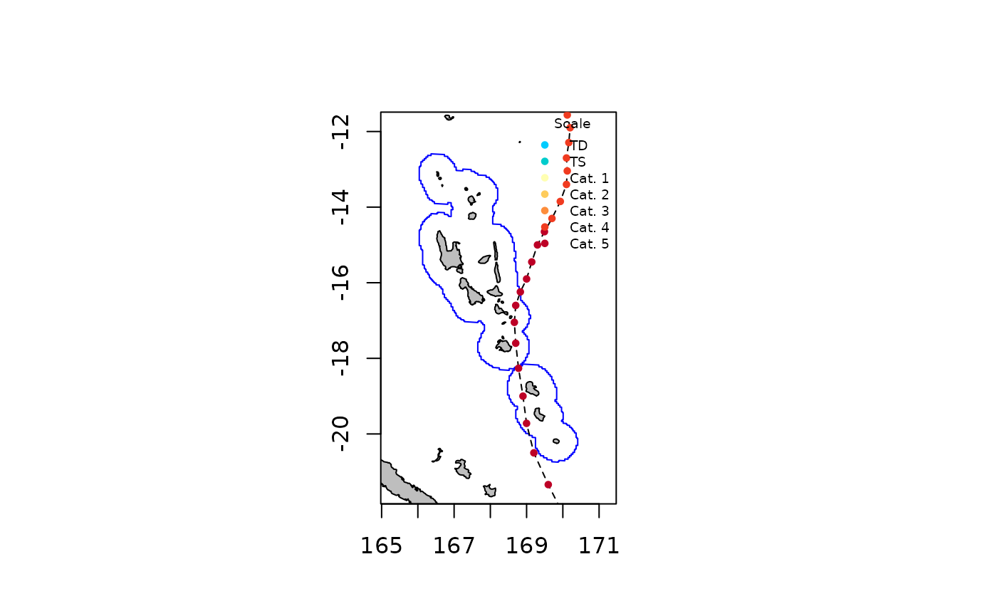

Exctracting topography

Then a Digital Terrain Model (DTM) is essential to compute topographic exposure to wind (TEW). In this tutorial, DTM used is Copernicus DEM30 data and is extracted thanks to the openEO package as follows :

library(openeo)
# connect to the backend and authenticate (an account is requirred)
connection <- connect(host = "https://openeofed.dataspace.copernicus.eu")
login()

# get the process collection to use the predefined processes of the back-end
p <- processes()

# define wanted data
data <- p$load_collection(
  id = "COPERNICUS_30",
  spatial_extent = list(
    west = 168.982086,
    south = -19.002400,
    east = 169.348755,
    north = -18.614363
  ),
  bands = c("DEM")
)


result <- p$save_result(data = data, format = "GTiff")

# save the tif file
compute_result(graph = result, output_file = "../filepath/name.tif")

Here, a sample DTM of Erromango Island included in StormR can be used:

dtm <- rast(system.file("extdata","test_datadtm.tif",package = "StormR"))

Other DTM / elevation products should work seemlessly with StormR.

Extracting spatial profiles

Spatial profiles must be computed prior to run the computeTEW() function.

spProfiles <- spatialBehaviour(st, product = "Profiles", verbose = 0)
spProfiles

## class       : SpatRaster
## size        : 196, 105, 36  (nrow, ncol, nlyr)
## resolution  : 0.04166667, 0.04166667  (x, y)
## extent      : 166.0417, 170.4167, -20.75, -12.58333  (xmin, xmax, ymin, ymax)
## coord. ref. : lon/lat WGS 84 (CRS84) (OGC:CRS84)
## source(s)   : memory
## names       : PAM_Speed_38, PAM_S~38.33, PAM_S~38.67, PAM_Speed_39, PAM_S~39.33, PAM_S~39.67, ...
## min values  :        7.494,       2.845,       2.253,        2.174,       4.195,       2.476, ...
## max values  :       74.833,   77.015999,   78.636002,    80.294998,   81.167999,   79.678001, ...
## time        : 2015-03-13 03:00:00 to 2015-03-13 20:00:00 (18 steps)

Other spatial profiles can be used as long as the layers of the spatRaster respect the following terminology : the name of the storm in capital letters, “Speed” or “Direction”, and the indices of the observation separated by underscores (e.g., “PAM_Speed_41”, “PAM_Direction_41”, …).

Topographic exposure to wind profiles

Using track data and the computeTEW() function with the product="TEW1wd" or product="TEW" argument we can generate topographic exposure fields at any time as follows:

pf <- computeTEW(spProfiles, st, dtm, product = "TEW", verbose = 0)
pf

## class       : SpatRaster
## size        : 479, 461, 18  (nrow, ncol, nlyr)
## resolution  : 0.0008102711, 0.0008100919  (x, y)
## extent      : 168.9787, 169.3522, -19.0037, -18.61566  (xmin, xmax, ymin, ymax)
## coord. ref. : lon/lat WGS 84 (EPSG:4326)
## source(s)   : memory
## varnames    : test_datadtm
##               test_datadtm
##               test_datadtm
##               test_datadtm
##               test_datadtm
##               ...
## names       : PAM_TEW_38, PAM_T~38.33, PAM_T~38.67, PAM_TEW_39, PAM_T~39.33, PAM_T~39.67, ...
## min values  :  -0.582549,   -0.682415,   -0.682448,  -0.681642,   -0.680588,   -0.678863, ...
## max values  :   0.713665,    0.853548,    0.852007,   0.854102,    0.854924,    0.855274, ...

The product TEW1wd compute TEW from one and only one wind direction taken at maximal wind speed location for the entire location of interest. This option should be used for small locations of interest, where wind direction is considered homogeneous.

On the other hand, TEW option computes TEW from one direction per pixel. This gives a more accurate picture for large scale areas where wind direction variations are important.

Multiple products can be computed at the same time, by simply providing a vector of product names, e.g. product = c("TEW1wd", "TEW").

The function returns a SpatRaster one raster for each observation or interpolated observation. Rasters’ names follow the following terminology, the name of the storm in capital letters, “TEW”, and the index of the observation, separated by underscores. Note that actual observations have entire indices (e.g., 41, 42, …) while interpolated observation have decimals (e.g., 41.1, 41.2, …). Most tropical cyclone track data sets are based on observations gathered every 3 or 6 hours. Therefore, to be able to compute wind fields every 1 hour, the observations are interpolated. This naming is coherent with spatialBehaviour and temporalBehaviour functions.

Topographic exposure profiles at the 41^th observation can be plotted as follows:

plotTEW(st, pf$PAM_TEW_41, dtm = dtm)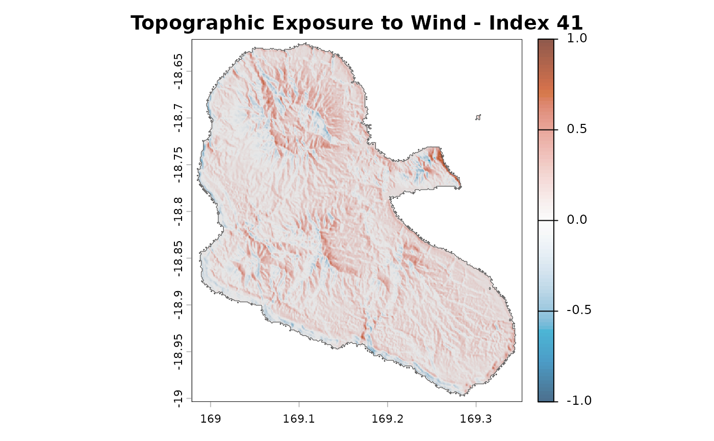

Topographic exposure to wind at specified locations

Topographic exposure to wind can also be computed at any location of interest.

This can be used in association with the temporalBehaviour function:

df <- data.frame(x = c(169.097), y = c(-18.723))
rownames(df) <- c("Forest Plot")
TS <- temporalBehaviour(st, points = df, product = "TS", tempRes = 30, verbose = 0)
pfTemp <- computeTEW(TS, df, dtm, verbose = 0)

And you can then plot the time series of the topographic exposure to wind at your location of interest as follows:

plotTemporalTEW(pfTemp, "PAM")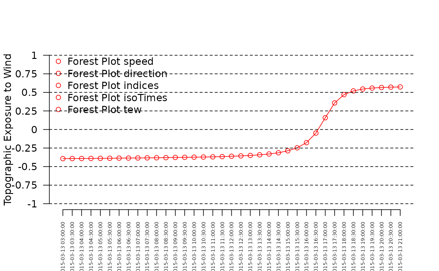

Summary Statistics

In addition to TEW at all observations time, the computeTEW() function can compute different “summary” products, either separately or together. “Summary” statistics are products integrated over the lifespan of the storm. Here, we compute all three integrated summary statistics together as follows:

ss <- computeTEW(spProfiles, st, dtm, product = c("TEW1wdMax", "TEW1wdMean", "TEWIntegrated"), verbose = 0)
ss

## class       : SpatRaster
## size        : 479, 461, 3  (nrow, ncol, nlyr)
## resolution  : 0.0008102711, 0.0008100919  (x, y)
## extent      : 168.9787, 169.3522, -19.0037, -18.61566  (xmin, xmax, ymin, ymax)
## coord. ref. : lon/lat WGS 84 (EPSG:4326)
## source(s)   : memory
## varnames    : 
##               
##               test_datadtm
## names       : PAM_TEW1wd_Max, PAM_TEW1wd_Mean, PAM_TEW_Integrated
## min values  :      -0.203111,       -0.494533,          -0.613323
## max values  :        0.85685,        0.657028,           0.773529

The computeTEW() function returns a SpatRaster object with three rasters:

one for the maximum TEW ("TEW1wd_Max"): TEW is computed for each time step using “Profiles” and only one wind direction (associated with the maximum wind speed for each layer of “Profiles”), and the the maximum value is return for each pixel.
one for the mean TEW ("TEW1d_Mean"): TEW is computed for each time step using “Profiles”, and only one wind direction (associated with the maximum wind speed for each layer of “Profiles”), and the the mean value is return for each pixel.
one for the maximum speed for each pixel TEW ("TEW_Integrated"): TEW is computed using wind direction associated with maximum wind speed over the whole lifespan of the storm for each pixel.

names(ss)

## [1] "PAM_TEW1wd_Max"     "PAM_TEW1wd_Mean"    "PAM_TEW_Integrated"

The maximum topographic exposure can be plotted as follows:

plotTEW(st, ss$PAM_TEW1wd_Max, dtm = dtm)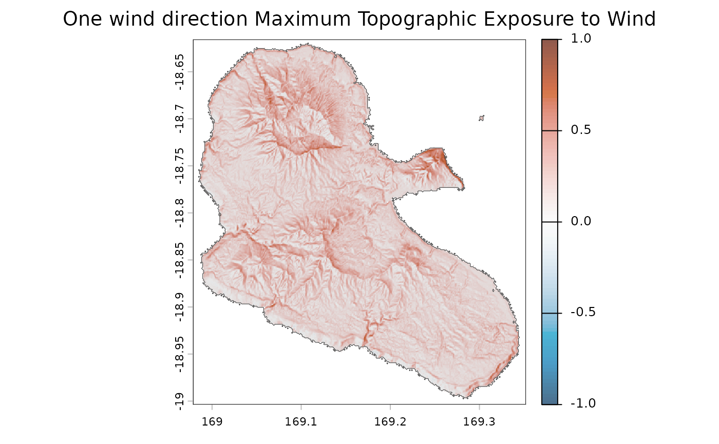

The mean topographic exposure can be plotted as follows:

plotTEW(st, ss$PAM_TEW1wd_Mean, dtm = dtm)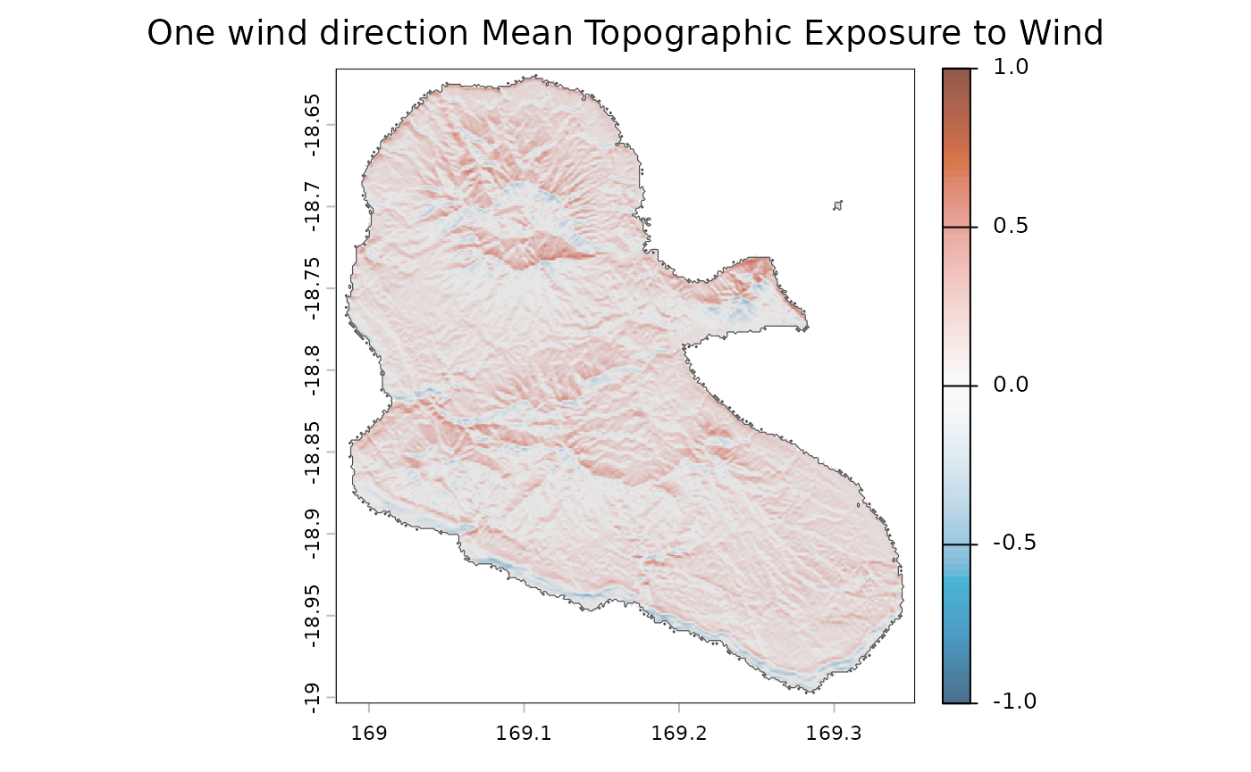

The summary of topographic exposure can be plotted as follows:

plotTEW(st, ss$PAM_TEW_Integrated, dtm = dtm)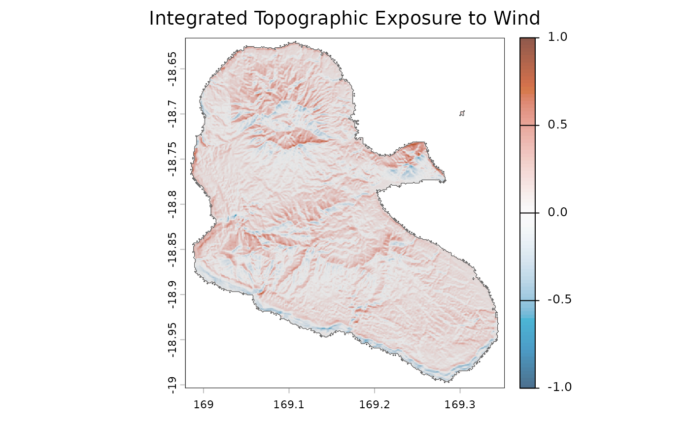

Dynamic plot

plotTEW function also provide (See ExtractStorms vignette) a dynamic plot. Here is an example based on the same parameters as above.

plotTEW(st, ss$PAM_TEW_Integrated, dtm = dtm, dynamicPlot = TRUE)

Exporting computeTEW products

The computeTEW() function returns rasters stored in a SpatRaster object than can be exported either in “.tiff” or “.nc” (NetCDF) formats using the writeRast() function. Here, we export the topographic exposure to wind in the working directory as follows:

writeRast(ss$PAM_TEW_Integrated)

Example of application : computing the Exposure Vulnerability Index

The time-series layers produced by computeTEW() (e.g., one layer per observation time from “TEW” or “TEW1wd” products) can be post-processed to build advanced ecological proxies. For instance, following the methodology defined by McLaren et al. (2019), Exposure Vulnerability (EV) can be computed to a specific storm or set of storms.

$EV = \frac{\sum_{i=1}^{n} (\text{MSW}_i \times \text{TEW}_i)}{n}$

It can be computed as follows :

# align msw on dtm
msw <- mask(project(spProfiles[[grep("_Speed", names(spProfiles))]], dtm), dtm)
# normalise
rg <- global(pf, c("min", "max"), na.rm = TRUE)
tew <- (pf - min(rg$min)) / (max(rg$max) - min(rg$min))

ev <- app(msw * tew, mean, na.rm = TRUE)

High EV index values indicate critical vulnerability zones, highlighting areas at peak risk for severe forest canopy damage and mechanical disturbance.

The EV index can be plotted as follows :

plot(ev, col = col)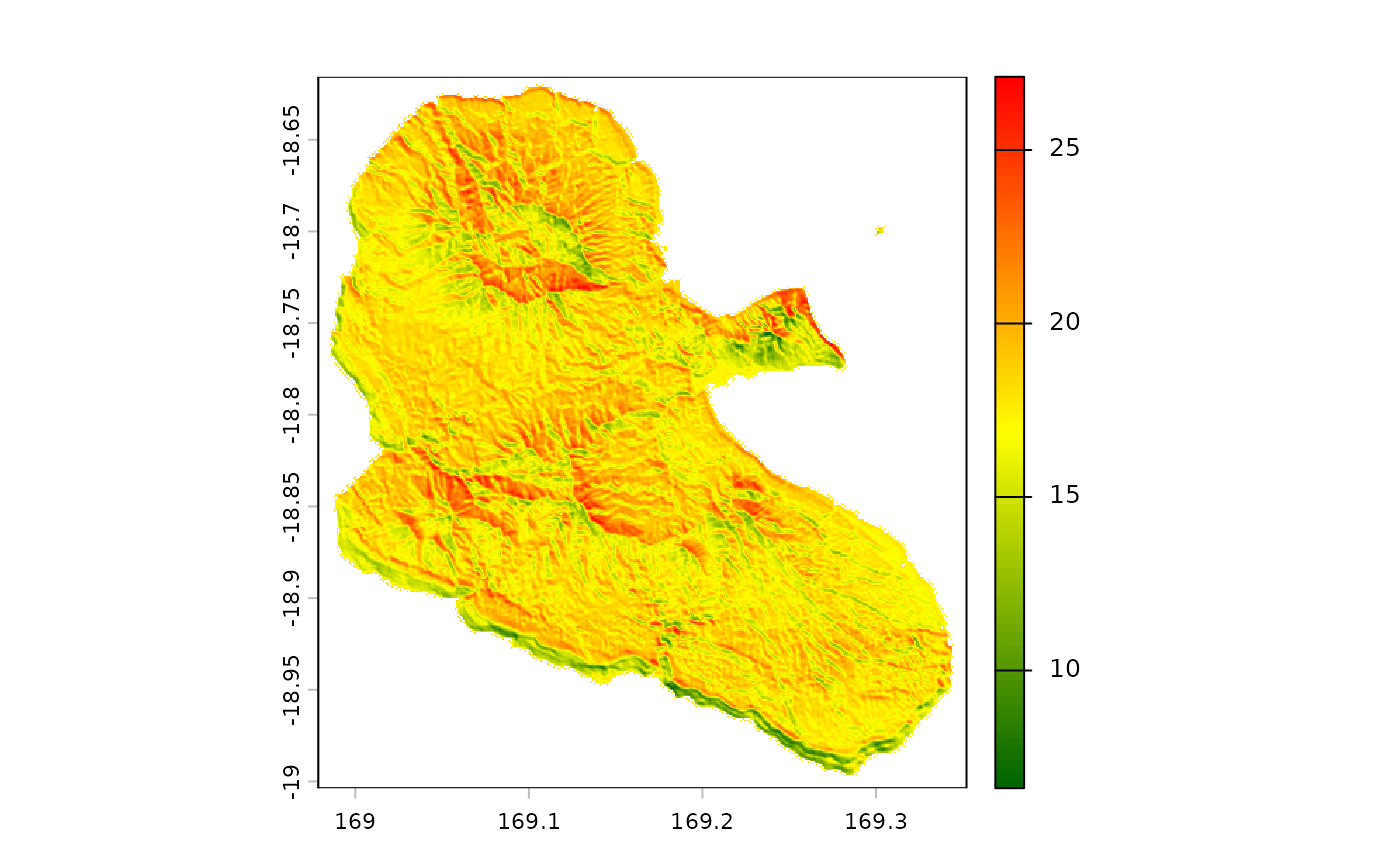

This cumulative index can be an extended landscape-scale predictor for long-term forest dynamics.

References

Boose, Emery R., David R. Foster, and Marcheterre Fluet. 1994. “Hurricane Impacts to Tropical and Temperate Forest Landscapes.” Ecological Monographs 64 (4): 369–400. https://doi.org/10.2307/2937142.

McLaren, K., D. Luke, E. Tanner, Peter J. Bellingham, and John R. Healey. 2019. “Reconstructing the Effects of Hurricanes over 155 Years on the Structure and Diversity of Trees in Two Tropical Montane Rainforests in Jamaica.” Agricultural and Forest Meteorology 276 (October). https://doi.org/10.1016/j.agrformet.2019.107621.

2026-06-30