Above-Ground Biomass Estimation with BIOMASS Package • CafriplotsR

Overview

This vignette demonstrates how to use CafriplotsR with the BIOMASS package to estimate above-ground biomass (AGB) for permanent forest plots. The query_plots() function with output_style = "permanent_plot" provides data structures optimized for allometric analyses.

Key advantages of the integrated workflow:

Automatic trait enrichment - Wood density and other traits are pre-integrated
Ready-made height-diameter table - $height_diameter table provided by default
Structured output - Separate tables for metadata, individuals, and measurements
Taxonomic hierarchies - Trait inheritance from species → genus → family

Prerequisites

library(CafriplotsR)
library(BIOMASS)
library(dplyr)
library(ggplot2)

# Connect to database
mydb <- call.mydb()
mydb_taxa <- call.mydb.taxa()

Step 1: Extract Plot Data

Use output_style = "permanent_plot" to get structured output optimized for biomass analysis:

# Query permanent plots with individual data
plot_data <- query_plots(
  plot_name = c("bouamir001", "mbalmayo001"),  # Example plots
  extract_individuals = TRUE, ## extract individuals/stems
  method = "1ha-IRD",
  con = mydb, 
  census_strategy = "first", ## get first census (if more than one) - in this case, because tree heights were measure during the first census
  ## If wd is not available for species, the mean of wd per genus is attributed to species belonging to this genus
  ## if wd if not available at genus level, plot mean is given
  ## generate a column that indicates the source of information
  traits_to_genera = TRUE 
)
#> ── Building plot filter query ──────────────────────────────────────────────────
#> ℹ Attempt 1 of 10...
#> ✔ ✅ Successfully connected and fetched 2 rows.
#> 
#> ── Querying plot features ──
#> 
#> ✔ Found 115 feature(s) for 2 plot(s)
#> ℹ Enriching with subplot observation features
#> 
#> ── Aggregating features to wide format ──
#> 
#> ✔ Query completed
#> ── Processing individuals ──────────────────────────────────────────────────────
#> ℹ Selected first census date column: date_census_1
#> ℹ Fetching individuals
#> ✔ Processed 888 individuals
#> ── Processing traits ───────────────────────────────────────────────────────────
#> ℹ Enriching with individual-level traits
#> 
#> ── Fetching individual features ──
#> 
#> ── Fetching trait measurements ──
#> 
#> ℹ Removed 283 measurement(s) with issues
#> ℹ Enriching with census information for first census selection
#> ✔ Selected first census for 2 plot(s)
#> ℹ Filtered out 3683 measurement(s) from other censuses
#> ✔ Query completed: 6110 measurement(s)
#> 
#> ── Aggregating features by individual ──
#> 
#> ℹ Aggregating 4597 numeric measurement(s)
#> ℹ Aggregating 1513 character measurement(s)
#> ✔ Aggregated 888 individual(s)
#> ℹ Enriching with taxonomic-level traits
#> 
#> ── Querying taxa-level traits ──
#> 
#> ℹ Fetching trait measurements for 154 taxon/taxa
#> ✔ Found 2790 measurement(s) for 140 taxa
#> ℹ Resolving taxonomic synonyms
#> 
#> ── Processing traits to wide format ──
#> 
#> ℹ Aggregating numeric traits
#> ℹ Aggregating categorical traits (mode)
#> ✔ Query completed
#> ✔ Added 12 numeric taxonomic trait column(s)
#> ✔ Added 14 categorical taxonomic trait column(s)
#> ℹ Aggregating traits to genus level
#> ℹ Source information added to columns starting with 'source_'
#> ℹ Attempt 1 of 10...
#> ✔ ✅ Successfully connected and fetched 10164 rows.
#> ℹ Attempt 1 of 10...
#> ✔ ✅ Successfully connected and fetched 6084 rows.
#> 
#> ── Querying taxa-level traits ──
#> 
#> ℹ Fetching trait measurements for 13017 taxon/taxa
#> ✔ Found 14335 measurement(s) for 2369 taxa
#> ℹ Resolving taxonomic synonyms
#> ℹ Including synonyms: 2369 taxa expanded to 5858 taxa
#> ℹ Adding taxonomic information
#> ✔ Query completed
#> ℹ Setting wood density SD to averaged species and genus level according to BIOMASS dataset
#> ! ids removed - remove_ids = TRUE
#> ℹ Auto-detected output style: 'permanent_plot' based on method field
#> ✔ Output restructured using 'permanent_plot' style. Use names() to see available tables.


# Check structure
names(plot_data)
#> [1] "metadata"        "individuals"     "height_diameter"
# $metadata - Plot-level information
# $individuals - Individual tree data with traits
# $height_diameter - Height-diameter pairs (ready for modeling)

The permanent_plot output style provides:

$metadata: Plot coordinates, area, census dates, investigators
$individuals: Complete tree inventory with taxonomic traits
$height_diameter: Pre-filtered height-diameter pairs for allometric modeling

Step 2: Explore the Data

Individual Tree Data

The individuals table includes automatically enriched traits:

# Check what data we have
str(plot_data$individuals)
#> tibble [888 × 19] (S3: tbl_df/tbl/data.frame)
#>  $ id_n                           : int [1:888] 248314 248318 248322 248326 248330 248334 248338 248342 248346 248350 ...
#>  $ plot_name                      : chr [1:888] "bouamir001" "bouamir001" "bouamir001" "bouamir001" ...
#>  $ tag                            : num [1:888] 1 2 3 4 5 6 7 8 9 10 ...
#>  $ family                         : chr [1:888] "Annonaceae" "Lecythidaceae" "Olacaceae" "Annonaceae" ...
#>  $ genus                          : chr [1:888] "Xylopia" "Petersianthus" "Heisteria" "Greenwayodendron" ...
#>  $ species                        : chr [1:888] "Xylopia quintasii" "Petersianthus macrocarpus" "Heisteria parvifolia" "Greenwayodendron suaveolens" ...
#>  $ dbh                            : num [1:888] 17.7 62.4 57.7 25.9 22.8 ...
#>  $ quadrat                        : chr [1:888] "0_0" "0_0" "0_0" "0_0" ...
#>  $ height                         : num [1:888] 12.8 NA NA NA NA ...
#>  $ census_date                    : Date[1:888], format: "2018-12-02" "2018-12-02" ...
#>  $ taxa_mean_wood_density         : num [1:888] 0.76 0.68 0.668 0.668 0.55 ...
#>  $ taxa_n_wood_density            : num [1:888] 5 10 NA NA 1 NA 3 1 4 1 ...
#>  $ taxa_sd_wood_density           : num [1:888] 0.0708 0.0708 0.0796 0.0796 0.0708 ...
#>  $ source_taxa_mean_wood_density  : chr [1:888] "species" "species" "plot_mean" "plot_mean" ...
#>  $ source_taxa_n_wood_density     : chr [1:888] "species" "species" NA NA ...
#>  $ source_taxa_sd_wood_density    : chr [1:888] "species" "species" "plot_mean" "plot_mean" ...
#>  $ taxa_sd_wood_density_plot_level: num [1:888] 0.0796 0.0796 0.0796 0.0796 0.0796 ...
#>  $ pom                            : num [1:888] 1.3 1.3 1.3 1.3 1.3 1.3 1.3 1.8 3.3 1.3 ...
#>  $ observations                   : chr [1:888] NA "rejets" NA NA ...

# Key columns for biomass:
# - dbh (stem_diameter): Diameter at breast height (cm)
# - species (tax_sp_level): Species name
# - wood_density_mean (taxa_mean_wood_density): Mean wood density (g/cm³)
# - wood_density_sd (taxa_sd_wood_density): SD for error propagation
# - source_taxa_mean_wood_density (taxa_sd_wood_density): source of information for wood density

# Summary of wood density availability
plot_data$individuals %>%
  summarise(
    n_total = n(),
    n_with_wd = sum(!is.na(taxa_mean_wood_density)),
    pct_with_wd = round(100 * n_with_wd / n_total, 1),
    mean_wd = mean(taxa_mean_wood_density, na.rm = TRUE)
  )
#> # A tibble: 1 × 4
#>   n_total n_with_wd pct_with_wd mean_wd
#>     <int>     <int>       <dbl>   <dbl>
#> 1     888       888         100   0.691

Note: Wood density traits are automatically: - Retrieved from the taxa database - Inherited from species → genus → family when species-level data unavailable - Averaged at plot level when no taxonomic match found (if traits_to_genera = TRUE)

Height-Diameter Data

The $height_diameter table is pre-filtered and ready for modeling:

# Height-diameter pairs (automatically filtered)
head(plot_data$height_diameter)
#> # A tibble: 6 × 6
#>     id_n plot_name    tag     D     H   POM
#>    <int> <chr>      <dbl> <dbl> <dbl> <dbl>
#> 1 248314 bouamir001     1  17.7  12.8   1.3
#> 2 248334 bouamir001     6  22.2  15.7   1.3
#> 3 248342 bouamir001     8  38.4  28.4   1.8
#> 4 248346 bouamir001     9 123.   40.4   3.3
#> 5 248370 bouamir001    15  48.7  25.8   1.3
#> 6 248410 bouamir001    25  11.2  10.5   1.3

# This table includes:
# - id_n: Individual ID
# - plot_name: Plot identifier
# - tag: Tree tag
# - D: Diameter (dbh in cm)
# - H: Height (tree height in m)
# - POM: Point of measurement (if available)

# Summary
plot_data$height_diameter %>%
  group_by(plot_name) %>%
  summarise(
    n_pairs = n(),
    mean_dbh = round(mean(D), 1),
    mean_height = round(mean(H), 1),
    dbh_range = paste(round(min(D), 1), "-", round(max(D), 1)),
    height_range = paste(round(min(H), 1), "-", round(max(H), 1))
  )
#> # A tibble: 2 × 6
#>   plot_name   n_pairs mean_dbh mean_height dbh_range    height_range
#>   <chr>         <int>    <dbl>       <dbl> <chr>        <chr>       
#> 1 bouamir001       76     28.9        20.4 10.9 - 122.9 8.9 - 40.4  
#> 2 mbalmayo001      46     33.2        24.7 10.3 - 134   10.7 - 41.1

Step 3: Build Height-Diameter Models

Use the pre-filtered $height_diameter table directly with BIOMASS:

Option A: Single Model (All Plots)

# Fit global height-diameter model
hd_model_global <- BIOMASS::modelHD(
  D = plot_data$height_diameter$D,
  H = plot_data$height_diameter$H,
  method = "weibull",
  useWeight = TRUE
)

# Check model fit
summary(hd_model_global)
#>              Length Class  Mode     
#> input          2    -none- list     
#> model          6    nls    list     
#> residuals    122    -none- numeric  
#> coefficients  12    -none- numeric  
#> R.squared      0    -none- NULL     
#> formula        7    -none- call     
#> method         1    -none- character
#> predicted    122    -none- numeric  
#> RSE            1    -none- numeric

# Residual Standard Error for uncertainty propagation
RSE_global <- hd_model_global$RSE
print(paste("RSE:", round(RSE_global, 3)))
#> [1] "RSE: 5.029"

Option B: Plot-Specific Models

For plots with sufficient height measurements (>15 pairs recommended):

# Build separate models per plot
hd_models_by_plot <- plot_data$height_diameter %>%
  group_by(plot_name) %>%
  filter(n() >= 15) %>%  # Require at least 15 H-D pairs
  group_split() %>%
  lapply(function(plot_df) {
    tryCatch({
      model <- BIOMASS::modelHD(
        D = plot_df$D,
        H = plot_df$H,
        method = "weibull",
        useWeight = TRUE
      )
      list(
        plot_name = unique(plot_df$plot_name),
        model = model,
        RSE = model$RSE,
        n = nrow(plot_df)
      )
    }, error = function(e) {
      NULL  # Return NULL if model fails
    })
  }) %>%
  Filter(Negate(is.null), .)  # Remove failed models

# Summary
cat(sprintf("Built %d plot-specific models\n", length(hd_models_by_plot)))
#> Built 2 plot-specific models

Visualize H-D Relationships

# Plot height-diameter data with fitted curve
ggplot(plot_data$height_diameter, aes(x = D, y = H)) +
  geom_point(aes(color = plot_name), alpha = 0.6, size = 2) +
  geom_smooth(method = "nls",
              formula = y ~ a * (1 - exp(-b * x^c)),
              method.args = list(start = list(a = 40, b = 0.05, c = 1)),
              se = TRUE, color = "black", linewidth = 1.5) +
  labs(
    title = "Height-Diameter Relationship",
    x = "Diameter at breast height (cm)",
    y = "Tree height (m)",
    color = "Plot"
  ) +
  theme_minimal() +
  theme(legend.position = "bottom")
#> Warning: Failed to fit group -1.
#> Caused by error in `pred$fit`:
#> ! $ operator is invalid for atomic vectors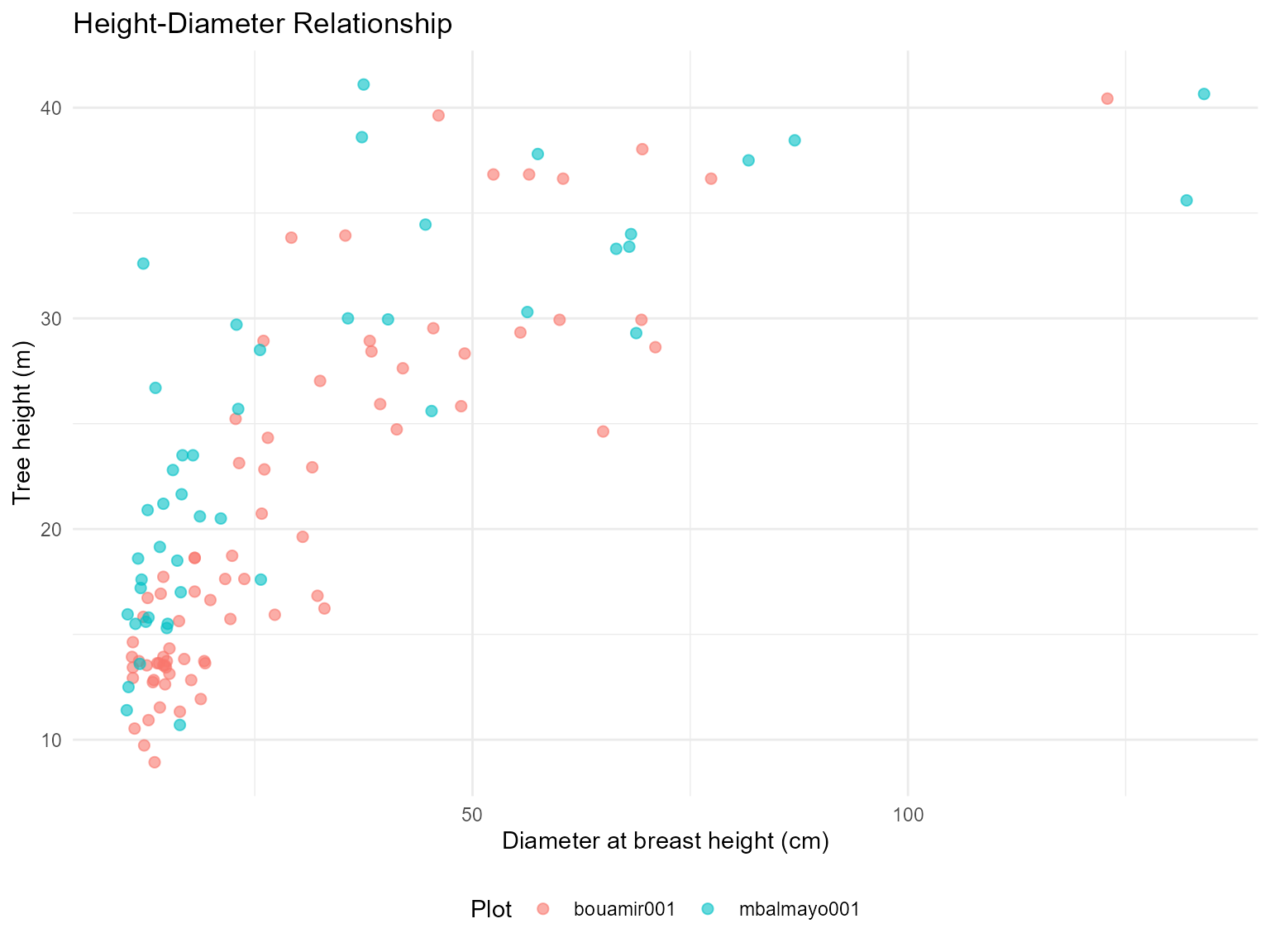

Step 4: Predict Missing Heights

Most trees don’t have height measurements. Use the H-D model to predict them:

# Prepare data for AGB estimation
agb_data <- plot_data$individuals %>%
  filter(!is.na(dbh)) %>%  # Must have diameter
  mutate(
    # Predict height using global model (or plot-specific if available)
    H_predicted = BIOMASS::retrieveH(
      D = dbh,
      model = hd_model_global
    )$H,
    # Use measured height if available, otherwise predicted
    H_final = ifelse(!is.na(height), height, H_predicted),
    # Assign RSE for uncertainty
    H_RSE = RSE_global
  )

# Check prediction success
agb_data %>%
  summarise(
    n_total = n(),
    n_measured = sum(!is.na(height)),
    n_predicted = sum(is.na(height)),
    pct_predicted = round(100 * n_predicted / n_total, 1)
  )
#> # A tibble: 1 × 4
#>   n_total n_measured n_predicted pct_predicted
#>     <int>      <int>       <int>         <dbl>
#> 1     834        122         712          85.4

Using plot-specific models (if available):

# Create lookup for plot-specific RSE
plot_rse <- data.frame(
  plot_name = sapply(hd_models_by_plot, function(x) x$plot_name),
  RSE_plot = sapply(hd_models_by_plot, function(x) x$RSE)
)

# Predict with plot-specific models where available
agb_data <- agb_data %>%
  filter(!is.na(dbh)) %>%
  left_join(plot_rse, by = "plot_name") %>%
  mutate(
    # Use plot-specific RSE if available, otherwise global
    H_RSE = ifelse(!is.na(RSE_plot), RSE_plot, RSE_global),
    # Predict heights (would need to loop through plot-specific models)
    H_final = ifelse(!is.na(height), height, H_predicted)
  )

Step 5: Estimate Above-Ground Biomass

Now we have all required inputs for BIOMASS:

D: Diameter (dbh)
WD: Wood density (automatically from database!)
H: Height (measured or predicted)
Errors: SD for wood density, RSE for height

Check Data Completeness

# Summary of required variables
summary(agb_data[, c("dbh", "taxa_mean_wood_density", "H_final", "H_RSE")])
#>       dbh        taxa_mean_wood_density    H_final          H_RSE      
#>  Min.   : 10.0   Min.   :0.2400         Min.   : 8.93   Min.   :4.280  
#>  1st Qu.: 12.3   1st Qu.:0.6400         1st Qu.:16.39   1st Qu.:4.280  
#>  Median : 16.2   Median :0.7100         Median :19.07   Median :5.299  
#>  Mean   : 23.3   Mean   :0.6912         Mean   :20.97   Mean   :4.824  
#>  3rd Qu.: 24.8   3rd Qu.:0.8000         3rd Qu.:23.86   3rd Qu.:5.299  
#>  Max.   :175.0   Max.   :0.9300         Max.   :41.10   Max.   :5.299

# Check for missing data
agb_data %>%
  summarise(
    missing_dbh = sum(is.na(dbh)),
    missing_wd = sum(is.na(taxa_mean_wood_density)),
    missing_height = sum(is.na(H_final)),
    complete_cases = sum(!is.na(dbh) & !is.na(taxa_mean_wood_density) & !is.na(H_final))
  )
#> # A tibble: 1 × 4
#>   missing_dbh missing_wd missing_height complete_cases
#>         <int>      <int>          <int>          <int>
#> 1           0          0              0            834

Single AGB Estimate (No Error Propagation)

Quick estimate without uncertainty:

# Simple AGB calculation using Chave et al. 2014 equation
agb_data <- agb_data %>%
  filter(!is.na(dbh) & !is.na(taxa_mean_wood_density) & !is.na(H_final)) %>%
  mutate(
    AGB_kg = BIOMASS::computeAGB(
      D = dbh,
      WD = taxa_mean_wood_density,
      H = H_final
    )
  )

# Plot-level AGB
agb_by_plot <- agb_data %>%
  group_by(plot_name) %>%
  summarise(
    n_trees = n(),
    total_AGB_Mg = sum(AGB_kg)
  )

print(agb_by_plot)
#> # A tibble: 2 × 3
#>   plot_name   n_trees total_AGB_Mg
#>   <chr>         <int>        <dbl>
#> 1 bouamir001      389         350.
#> 2 mbalmayo001     445         466.

Summary

This vignette demonstrated the complete workflow for AGB estimation using CafriplotsR and BIOMASS:

✅ Extract structured data with output_style = "permanent_plot"
✅ Use pre-filtered H-D data from $height_diameter table
✅ Build allometric models with BIOMASS::modelHD()
✅ Leverage integrated traits - wood density automatically included

Key advantages:

No manual trait matching - wood density pre-integrated from taxa database
Ready-made H-D table - filtered and formatted for BIOMASS

Additional Resources

BIOMASS package: Réjou-Méchain et al. (2017) https://CRAN.R-project.org/package=BIOMASS
Allometric equations: Chave et al. (2014) https://doi.org/10.1111/gcb.12629
CafriplotsR queries: See vignette("using-query-plots")
Taxonomic matching: See vignette("taxonomic-app")

References

Chave, J., et al. (2014). Improved allometric models to estimate the aboveground biomass of tropical trees. Global Change Biology, 20(10), 3177-3190.

Réjou-Méchain, M., et al. (2017). biomass: an R package for estimating above-ground biomass and its uncertainty in tropical forests. Methods in Ecology and Evolution, 8(9), 1163-1167.